AFM vs SEM: A Comprehensive Guide to Choosing the Right Surface Characterization Tool for Biomedical Research
This article provides a detailed comparison of Atomic Force Microscopy (AFM) and Scanning Electron Microscopy (SEM) for surface characterization in biomedical and pharmaceutical research.
AFM vs SEM: A Comprehensive Guide to Choosing the Right Surface Characterization Tool for Biomedical Research
Abstract
This article provides a detailed comparison of Atomic Force Microscopy (AFM) and Scanning Electron Microscopy (SEM) for surface characterization in biomedical and pharmaceutical research. We explore the foundational principles of each technique, delve into their specific methodological applications for analyzing materials from drug carriers to biological tissues, address common troubleshooting and optimization challenges, and provide a direct, data-driven comparison of their capabilities for validation. Aimed at researchers and drug development professionals, this guide synthesizes current best practices to help you select the optimal tool for your specific research questions involving topography, mechanical properties, and nanoscale imaging.
AFM and SEM Demystified: Core Principles and When to Use Each Technique
This application note, framed within a broader thesis comparing Atomic Force Microscopy (AFM) and Scanning Electron Microscopy (SEM) for surface characterization, details the core mechanisms, applications, and protocols for these techniques. AFM utilizes a physical probe for nanoscale surface interaction, while SEM employs a focused electron beam for imaging. Understanding their fundamental differences is critical for researchers, particularly in material science and drug development, to select the optimal tool for specific research questions.
Core Mechanism Comparison
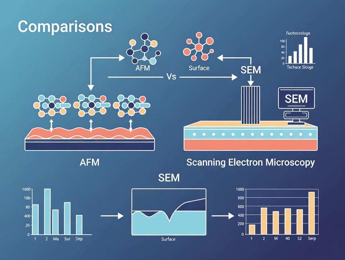
AFM (Physical Probe): A sharp tip on a cantilever scans the sample surface. Forces between the tip and the surface cause cantilever deflection, measured by a laser and photodetector. This feedback controls vertical movement, building a 3D topographic map. SEM (Electron Beam): A focused beam of high-energy electrons scans the sample. Interactions (e.g., secondary electron emission) are detected to generate a 2D intensity image representing surface morphology and composition.
Key Parameter Comparison Table
Table 1: Core Imaging Parameter Comparison for AFM vs. SEM
| Parameter | Atomic Force Microscopy (AFM) | Scanning Electron Microscopy (SEM) |
|---|---|---|
| Probe/Source | Physical tip (Si, SiN) | Focused beam of electrons |
| Resolution | Atomic (~0.1 nm vertical, ~1 nm lateral) | ~0.5 nm to 5 nm (depends on mode and voltage) |
| Working Environment | Ambient air, liquid, vacuum | High vacuum typically (ESEM allows hydrated samples) |
| Sample Requirements | Minimal preparation; conductive & non-conductive | Often requires conductive coating for non-conductive samples |
| Imaging Dimension | True 3D topography (height data) | 2D projection image (3D via stereo-pair or FIB-SEM) |
| Primary Data | Surface height, mechanical properties (e.g., modulus) | Surface morphology, composition (with EDS), crystallography |
| Maximum Sample Size | ~10s of cm (depends on stage) | ~10s of cm (depends on chamber) |
| Imaging Depth | Surface only (topography) | Surface and near-surface (interaction volume ~µm) |
| Key Applications | Roughness, force spectroscopy, live-cell imaging, nanotribology | High-throughput surface inspection, particle analysis, failure analysis |
| Typical Cost | $$ - $$$ | $$$ - $$$$ |
Table 2: Performance Metrics in Common Research Scenarios
| Research Scenario | Optimal Tool | Typical Resolution Achieved | Key Measurable Output |
|---|---|---|---|
| Polymer Surface Nanostructure | AFM (Tapping Mode) | 5-10 nm lateral | RMS Roughness, pore size distribution, phase imaging |
| Metal Fracture Surface Analysis | SEM | 1-3 nm | Crack morphology, grain structure, elemental analysis (via EDS) |
| Lipid Bilayer or Membrane Protein | AFM (Liquid Cell) | 1-5 nm lateral | Molecular arrangement, mechanical properties, real-time dynamics |
| Nanoparticle Size & Morphology | SEM | 0.5-2 nm | Particle diameter (count > 100), shape classification, aggregation state |
| Live Cell Surface Dynamics | AFM (Bio-AFM) | 10-50 nm lateral | Cell stiffness (Young's modulus), receptor mapping, morphological changes |
Experimental Protocols
Protocol 1: AFM for Topographical Imaging of a Pharmaceutical Powder (Contact Mode)
Objective: To obtain high-resolution 3D topography and surface roughness measurements of an active pharmaceutical ingredient (API) to assess batch consistency.
Materials: See "The Scientist's Toolkit" below.
Method:
- Sample Preparation: Lightly dust the API powder onto a double-sided adhesive carbon tab mounted on a standard AFM metal stub. Use compressed air to remove loose particles.
- Tip Mounting: Install a silicon nitride (SiN) tip for contact mode onto the tip holder. Carefully engage the tip holder into the AFM head.
- Loading & Alignment: Place the sample stub on the AFM stage. Align the laser spot to the end of the cantilever and adjust the photodetector to achieve a balanced signal.
- Engagement: Using the microscope's optical view, position the tip above a particle of interest. Initiate the automated engage sequence to bring the tip into gentle contact with the surface.
- Scan Parameter Setup: Set scan size to 5 µm x 5 µm. Adjust the setpoint to maintain a low, constant force (typically 0.5-5 nN). Set scan rate to 1-2 Hz.
- Image Acquisition: Initiate scanning. Adjust feedback gains to optimize tracking. Acquire both height and deflection channel images.
- Retraction & Data Saving: After scanning, retract the tip. Save the raw data file.
- Analysis: Use analysis software to level the image (flatten or plane fit) and calculate roughness parameters (Ra, Rq, Rz) over a defined area.
Protocol 2: SEM Imaging of a Drug-Eluting Stent Coating
Objective: To visualize the surface morphology and uniformity of a polymer coating on a metallic stent before and after in vitro elution testing.
Materials: See "The Scientist's Toolkit" below.
Method:
- Sample Preparation (Critical): Mount the stent segment on an SEM stub using conductive adhesive. For non-conductive polymer coating, sputter-coat the sample with a 5-10 nm layer of gold/palladium using a sputter coater.
- Chamber Evacuation: Insert the sample stub into the SEM load lock chamber. Evacuate the load lock, then transfer the sample to the main chamber. Allow the system to achieve high vacuum (<10⁻⁴ Pa).
- Microscope Initialization: Ensure the electron column is aligned. Select an accelerating voltage appropriate for the sample (5-10 kV for coated polymers to avoid charging and damage).
- Locating the Area of Interest: Use the stage controls and low-magnification imaging to navigate to the region of interest on the stent strut.
- Image Optimization: Adjust the working distance (e.g., 5-10 mm). Fine-tune focus and astigmatism correction. Select a suitable aperture size. Adjust brightness/contrast using the detector signal.
- Image Acquisition: Acquire micrographs at increasing magnifications (e.g., 500x, 5000x, 20,000x) to assess coating integrity at different scales. Use the secondary electron (SE) detector for topographical contrast.
- Optional EDS Analysis: If equipped, perform energy-dispersive X-ray spectroscopy (EDS) spot or area analysis to confirm coating composition or detect residual drug crystals.
- Sample Retrieval: Vent the chamber and retrieve the sample.
Visualizations
AFM Operational Workflow
SEM Signal Generation Pathway
AFM vs SEM Selection Guide
The Scientist's Toolkit
Table 3: Essential Research Reagents & Materials
| Item | Primary Function | Common Example / Specification |
|---|---|---|
| AFM Cantilever/Tip | Physical probe for surface interaction; different tips for different modes and properties. | Contact Mode: SiN tip (0.1-0.6 N/m). Tapping Mode: Si tip (20-80 N/m, ~10 nm radius). |
| Conductive Adhesive | To securely mount samples to AFM stubs or SEM holders while providing electrical grounding. | Double-sided carbon tape, silver paint, copper tape. |
| Sputter Coater | Deposits a thin, conductive metal layer onto non-conductive samples to prevent charging in SEM. | Gold/Palladium (Au/Pd) target, 5-15 nm coating thickness. |
| SEM Sample Stubs | Standardized mounts that hold samples in the SEM chamber. | Aluminum stubs (12.5 mm diameter) with various mounting pins. |
| Calibration Grids | Certified reference samples for verifying the lateral (XY) and vertical (Z) scale accuracy of AFM/SEM. | TGXYZ series (AFM), grating replicas (e.g., 1000 nm pitch), NIST-traceable standards. |
| Dust-Removing Gas | To clean samples and stages of particulate contamination without contact. | Canned, ultra-clean, oil-free compressed air or nitrogen. |
| AFM Liquid Cell | Enables imaging in controlled fluid environments for biological samples or electrochemical studies. | Sealed cell with O-rings and fluid inlet/outlet ports. |
| EDS Calibration Standard | Used to calibrate the Energy-Dispersive X-ray Spectrometer for quantitative elemental analysis. | Copper (Cu) or Cobalt (Co) block, or multi-element standard. |
This application note details key metrics for surface characterization in materials and life sciences, contextualized within the comparative analysis thesis of Atomic Force Microscopy (AFM) versus Scanning Electron Microscopy (SEM). AFM provides three-dimensional nanoscale data on physical properties, while SEM excels in high-resolution imaging and elemental composition. Selecting the appropriate technique is critical for research in drug delivery, biomaterials, and nano-formulation.
Key Metrics: AFM vs. SEM Capabilities
| Metric | What It Measures | Primary Technique | Typical Quantitative Output | Key Application in Drug Development |
|---|---|---|---|---|
| Topography | The three-dimensional shape and features of a surface. | AFM (Contact/Tapping Mode), SEM | Height (nm), Z-range (nm), lateral feature size (nm). | Visualizing particle morphology, coating uniformity, tablet surface defects. |
| Roughness | The deviations in surface height from an ideal plane; quantifies texture. | AFM (derived from topography) | Ra (Arithmetic Avg., nm), Rq (RMS, nm), Rz (Ten-point height, nm). | Correlating surface texture with adhesion, dissolution rates, and biocompatibility. |
| Modulus | Elasticity or stiffness; resistance to deformation. | AFM (Force Spectroscopy/Mapping) | Young's Modulus (kPa to GPa). | Measuring mechanical properties of cells, hydrogels, polymer matrices, and lipid nanoparticles. |
| Composition | Elemental or chemical identity of surface components. | SEM-EDS, AFM (advanced modes: IR, thermal, PFM) | Elemental maps (weight %), phase maps, adhesion maps. | Identifying contaminants, verifying coating composition, mapping API distribution in blends. |
Experimental Protocols
Protocol 1: AFM for Topography, Roughness, and Modulus on a Pharmaceutical Film
Objective: To characterize the surface morphology, roughness, and nanomechanical properties of a polymer-based drug-loaded film. Materials: AFM with cantilevers for tapping mode and force spectroscopy (nominal spring constant: 0.5-5 N/m, tip radius <10 nm), sample film, adhesive tape. Workflow:
- Sample Preparation: Affix the film to a standard AFM metal puck using double-sided adhesive tape. Ensure the surface is clean and free of particulates using gentle nitrogen gas flow.
- Topography & Roughness Scan:
- Mount the sample. Engage the cantilever in tapping mode.
- Scan a minimum of three (3) different 10 µm x 10 µm areas.
- Set scan rate to 0.5-1 Hz with 512 samples/line resolution.
- Apply first-order flattening to the raw height image.
- Use analysis software to calculate Ra and Rq over the entire image.
- Modulus Mapping via Force Spectroscopy:
- Switch to a cantilever calibrated for its exact spring constant (using thermal tune method).
- Perform a force-volume map over a 5 µm x 5 µm area (e.g., 32x32 points).
- At each point, record a force-distance curve with a trigger force of 5 nN.
- Fit the retract curve's contact region to the Derjaguin–Muller–Toporov (DMT) model to calculate Young's Modulus. Apply a Poisson's ratio assumption (e.g., 0.5 for soft materials).
Protocol 2: SEM-EDS for Topography and Composition of a Powder Blend
Objective: To image surface morphology and determine elemental composition of a powder blend containing an API (e.g., with distinctive elemental signature). Materials: Field-Emission SEM with EDS detector, conductive carbon tape, sputter coater (Au/Pd), aluminum stub. Workflow:
- Sample Preparation:
- Adhere conductive carbon tape to an aluminum stub.
- Sparingly sprinkle powder onto the tape. Use compressed air to remove loose particles.
- Sputter-coat the sample with a 5-10 nm layer of Au/Pd to prevent charging.
- SEM Imaging:
- Insert the sample. Pump the chamber to high vacuum (~10^-4 Pa).
- Select an accelerating voltage of 5-10 kV (optimal for surface detail and EDS).
- Acquire secondary electron (SE) images at various magnifications (e.g., 500x, 10,000x, 50,000x).
- EDS Compositional Analysis:
- At a region of interest (ROI), position the beam. Collect an EDS spectrum with a live time of 60 seconds.
- Use the instrument software to identify characteristic X-ray peaks (e.g., for elements like C, O, N, S, F).
- Acquire an elemental map for a distinctive element in the API (e.g., Sulfur) over a selected area. Set a dwell time of 100-200 µs/pixel.
Visualization
AFM vs SEM Decision Flow
AFM Force Curve Analysis Stages
The Scientist's Toolkit: Research Reagent Solutions
| Item | Function / Relevance |
|---|---|
| AFM Cantilevers (Tapping Mode) | Silicon probes with a resonant frequency for non-destructive imaging of soft samples (e.g., biologics, polymers). |
| AFM Cantilevers (Contact/Force) | Sharp tipless or spherical-tipped probes with calibrated spring constants for accurate modulus measurement. |
| Conductive Adhesive Tabs (Carbon Tape) | For mounting non-conductive samples to SEM stubs to prevent charging artifacts. |
| Sputter Coater with Au/Pd Target | Deposits a thin, conductive metal layer on insulating samples for high-quality SEM imaging. |
| Standard Reference Samples | Gratings (for AFM calibration), polymer films of known modulus, pure element blocks (for EDS calibration). |
| Vibration Isolation Table | Critical for AFM operation to dampen ambient acoustic and seismic noise for stable imaging. |
| High-Purity Nitrogen Gas | Used for dust-free sample cleaning and drying in sample preparation for both AFM and SEM. |
Within the comparative research framework of Atomic Force Microscopy (AFM) versus Scanning Electron Microscopy (SEM) for surface characterization, the hardware components define each technique's capabilities and limitations. AFM, a scanning probe technique, relies on mechanical interaction via a cantilever-tip system, while SEM employs electron optics within a vacuum chamber with specialized detectors. This note details these essential components, providing application protocols and comparative data for researchers in nanoscience and drug development.
Component Analysis & Comparative Data
Cantilevers & Tips (AFM Core)
The cantilever-tip system is the primary sensor in AFM. Its properties dictate resolution, imaging mode, and sample interaction.
Research Reagent Solutions: AFM Probes
| Item | Function & Explanation |
|---|---|
| Silicon Nitride Probes (e.g., MLCT-BIO) | Soft cantilevers (0.01-0.6 N/m) for bio-applications; minimize sample damage. |
| Silicon Probes (e.g., TAP150) | Stiffer cantilevers (~5 N/m) for tapping mode; high resonance frequency. |
| Conductive Diamond-Coated Tips | For electrical modes (SSRM, KPFM); wear-resistant. |
| Magnetic Coated Tips (e.g., MESP-HM) | For Magnetic Force Microscopy (MFM). |
| Functionalized Tips (e.g., PEG linkers) | Chemically modified for force spectroscopy (ligand-receptor binding studies). |
Table 1: Common AFM Cantilever Properties
| Cantilever Type | Spring Constant (N/m) | Resonance Frequency (kHz) | Typical Tip Radius | Primary Application |
|---|---|---|---|---|
| Contact Mode (Si₃N₄) | 0.01 - 0.5 | 5 - 60 | 20 nm | Soft sample imaging in liquid |
| Tapping Mode (Si) | 1 - 50 | 70 - 400 | 5 - 10 nm | High-res topography in air |
| Ultra-High Res (Si) | 10 - 80 | 200 - 800 | < 5 nm | Atomic-scale imaging |
| Bio-Lever Mini (Si) | 0.006 - 0.03 | 8 - 25 | 20 nm | Molecular force spectroscopy |
Protocol 1: Calibration of Cantilever Spring Constant via Thermal Tune Method Objective: Accurately determine the spring constant (k) of an AFM cantilever for quantitative force measurements. Materials: AFM with thermal tune software, cantilever, clean sample dish. Procedure: 1. Mount the cantilever securely in the holder and align the laser. 2. Retract the tip fully from any surface to avoid damping. 3. Acquire the thermal noise spectrum of the free cantilever. 4. Fit the fundamental resonance peak to a simple harmonic oscillator model. 5. Calculate k using the equipartition theorem: (k = kB T / \langle z^2 \rangle), where (kB) is Boltzmann's constant, T is temperature, and (\langle z^2 \rangle) is the mean squared deflection. 6. Record the calculated k and resonance frequency for experimental use.
Vacuum Chambers & Detectors (SEM Core)
The SEM requires a high-vacuum environment for its electron column and utilizes detectors to collect emitted signals from the sample.
Research Reagent Solutions: SEM Sample Preparation & Imaging
| Item | Function & Explanation |
|---|---|
| Sputter Coater (Gold/Palladium) | Deposits conductive nanolayer on insulating samples to prevent charging. |
| Critical Point Dryer | Preserves delicate, hydrated structures (e.g., biological tissues) for SEM via solvent replacement with CO₂. |
| Conductive Adhesive Tape | Mounts sample to stub; provides electrical ground path. |
| Carbon Paint | Alternative adhesive with high conductivity for stubborn charging issues. |
Table 2: Common SEM Detectors and Their Signals
| Detector Type | Signal Collected | Primary Information | Optimal Use Case |
|---|---|---|---|
| Everhart-Thornley (ETD) | Secondary Electrons (SE) | Topography, surface morphology | Standard high-vacuum imaging |
| In-Lens Detector | Secondary Electrons | High-resolution surface details | High-magnification work |
| Backscattered Electron (BSD) | Backscattered Electrons (BSE) | Atomic number contrast (composition) | Phase distribution, material contrast |
| Energy-Dispersive X-ray (EDS) | Characteristic X-rays | Elemental composition & mapping | Chemical analysis |
Protocol 2: Standard Sample Preparation for High-Vacuum SEM Imaging Objective: Render a non-conductive sample (e.g., polymer or biological specimen) suitable for high-resolution SEM without charging artifacts. Materials: SEM stub, conductive tape, sputter coater, desiccator. Procedure: 1. Mounting: Secure the sample to an aluminum stub using conductive carbon tape. Ensure a continuous path for electrons to ground. 2. Drying: For hydrated samples, perform sequential ethanol dehydration (e.g., 30%, 50%, 70%, 90%, 100%) followed by critical point drying. 3. Coating: Place the stub in a sputter coater. Pump down to low vacuum (~0.1 mbar). Coat the sample with a 5-10 nm layer of gold/palladium using a low current for 60-120 seconds. 4. Storage: Store coated samples in a desiccator until imaging to prevent moisture absorption. 5. Loading: Insert the stub into the SEM chamber, ensuring good electrical contact. Allow pump-down to high vacuum (<10⁻⁵ mbar) before imaging.
Integrated Workflow for Comparative Characterization
Title: Workflow for Choosing AFM vs SEM Based on Research Goal
The selection between AFM and SEM hinges on the specific hardware components and their corresponding data outputs. AFM's cantilever-tip system provides unparalleled 3D topography and quantitative nanomechanical data in ambient or liquid environments, crucial for dynamic biological studies. SEM's vacuum chamber and detector suite offer rapid, high-resolution surface imaging with elemental analysis, ideal for compositional mapping. A synergistic approach, leveraging both techniques' hardware strengths, provides the most comprehensive surface characterization platform for advanced materials and drug delivery system research.
Within a comparative thesis on Atomic Force Microscopy (AFM) and Scanning Electron Microscopy (SEM) for surface characterization, sample preparation is a critical differentiator. AFM generally operates under ambient to controlled atmospheric conditions, while SEM requires high vacuum (typically ≤10⁻⁴ Pa) for conventional imaging. This imposes fundamentally different constraints on sample handling, preparation, and compatibility. The choice of technique is often dictated by the sample's nature and its tolerance to these environmental extremes.
Environmental Requirements: A Quantitative Comparison
Table 1: Operational Environment and Sample Constraints for AFM vs. SEM
| Parameter | Atomic Force Microscopy (AFM) | Scanning Electron Microscopy (SEM) |
|---|---|---|
| Operational Pressure | Ambient air, controlled atmosphere (N₂, CO₂), liquid cells, or vacuum. | High vacuum (10⁻³ to 10⁻⁶ Pa) for conventional SEM. Variable Pressure/Low Vacuum (10-250 Pa) modes available. |
| Sample Conductivity Requirement | Not required. Can image insulators directly. | Essential for conventional high-vacuum SEM to prevent charging. Non-conductive samples require coating. |
| Maximum Sample Size (Typical) | ~10-20 cm diameter, limited by stage. Height: <10 cm. | ~10-30 cm diameter, limited by chamber. Height: <5-10 cm. |
| Sample State Compatibility | Solid surfaces, thin films, polymers, biomolecules in fluid, soft materials (e.g., gels). | Solid, dry, vacuum-compatible samples. Liquid samples require specialized cryogenic or capsule systems. |
| Primary Preparation Concern | Cleanliness, flatness, adhesion to substrate. | Conductivity, vacuum stability, outgassing, dehydration. |
Experimental Protocols
Protocol 1: Universal Sample Cleaning for AFM & SEM (Initial Step)
Objective: Remove particulate and hydrocarbon contamination. Materials: Cleanroom wipes, analytical grade solvents (acetone, ethanol, isopropanol), ultrasonic bath, dry nitrogen gun. Procedure:
- For rigid samples (silicon, metals), use a solvent sequence: soak in acetone for 5 minutes in an ultrasonic bath, followed by ethanol for 5 minutes.
- Rinse with fresh isopropanol.
- Dry immediately using a stream of dry, filtered nitrogen.
- For soft or sensitive samples, use gentle solvent rinses or piranha solution (H₂SO₄:H₂O₂ 3:1; EXTREME CAUTION) only for compatible, robust substrates like silicon.
Protocol 2: Sample Preparation for High-Resolution AFM in Air
Objective: Prepare a flat, clean substrate for nanoparticle or molecular imaging. Materials: Freshly cleaved mica (V1 grade), adhesive tape, 150 µM calcium chloride (CaCl₂) solution, biological sample in buffer. Procedure:
- Substrate Preparation: Cleave mica using adhesive tape to expose a fresh, atomically flat surface.
- Sample Deposition: Apply 20-50 µL of sample solution onto the mica. For biomolecules, add 10 µL of 150 µM CaCl₂ to improve adhesion.
- Incubation: Allow adsorption for 2-10 minutes.
- Rinsing & Drying: Rinse gently with 2 mL of ultrapure water to remove salts. Dry with a gentle stream of nitrogen.
Protocol 3: Sample Preparation for Conventional High-Vacuum SEM
Objective: Render a non-conductive sample (e.g., polymer, biological tissue) conductive and vacuum-stable. Materials: Sputter coater, carbon tape, aluminum stubs, conductive silver paint. Procedure:
- Mounting: Secure the sample to an aluminum stub using carbon tape. Ensure a continuous conductive path from sample top to stub.
- Electrical Connection: Apply a small amount of conductive silver paint between the sample edge and the stub.
- Coating: Place the stub in a sputter coater. Evacuate the coater to ~5 Pa.
- Sputtering: Deposit a 5-10 nm thin film of gold/palladium (Au/Pd) or platinum. Thicker coatings may obscure fine surface details.
- Storage: Store in a desiccator if not imaged immediately.
Workflow and Decision Pathway
Diagram Title: Decision Workflow: AFM vs SEM Sample Preparation
The Scientist's Toolkit: Essential Research Reagent Solutions
Table 2: Key Materials for Sample Preparation
| Item | Function | Typical Application |
|---|---|---|
| Freshly Cleaved Mica | Provides an atomically flat, negatively charged substrate for adsorption. | AFM of biomolecules (DNA, proteins), nanoparticles in air/liquid. |
| Conductive Carbon Tape | Provides both adhesion and electrical conductivity between sample and stub. | Mounting for SEM on aluminum stubs. |
| Au/Pd (80/20) Target | Source material for sputter coating; provides a fine-grained, conductive film. | Rendering non-conductive samples conductive for high-resolution SEM. |
| Conductive Silver Paint | Creates a low-resistance electrical path from sample surface to stub. | Supplementing carbon tape for SEM, especially for uneven samples. |
| Glutaraldehyde (2-5%) | Cross-linking fixative that preserves structure by binding proteins. | Fixing biological samples (cells, tissues) for SEM analysis. |
| Hexamethyldisilazane (HMDS) | A chemical drying agent that reduces surface tension and collapse. | Dehydrating and drying soft biological samples for SEM. |
| Piranha Solution | Removes organic residues aggressively; creates hydrophilic surface. | Ultra-cleaning silicon wafers or AFM tips (Highly Hazardous). |
| Polystyrene Beads (e.g., 100nm) | Calibration standard with known size and morphology. | Verifying scale and resolution of both AFM and SEM instruments. |
The selection of an imaging technique for surface characterization, particularly in materials science and life sciences, hinges on a fundamental trade-off. Atomic Force Microscopy (AFM) provides unparalleled three-dimensional topographical data and quantitative mechanical property mapping but at lower spatial resolution and slower scan speeds. Scanning Electron Microscopy (SEM) offers high-resolution, two-dimensional visual imaging with greater field of view and speed but lacks inherent quantitative mechanical data and requires specific sample preparation (e.g., conductive coating, vacuum compatibility). This Application Note details protocols and considerations for leveraging each technique within an integrated research framework.
Quantitative Comparison of Core Capabilities
Table 1: Comparative Metrics of AFM and SEM for Surface Characterization
| Parameter | Atomic Force Microscopy (AFM) | Scanning Electron Microscopy (SEM) |
|---|---|---|
| Resolution | Sub-nanometer vertical; ~1 nm lateral (in contact mode) | ~1 nm lateral (field emission); 1-20 nm typical |
| Imaging Environment | Ambient air, liquid, or controlled atmosphere; No vacuum required | High vacuum typically required (except for ESEM) |
| Sample Requirements | Minimal preparation; Conductive and non-conductive samples OK | Often requires conductive coating for non-conductive samples; Must be vacuum-stable |
| Data Type | 3D topographical map; Quantitative mechanical (modulus, adhesion), electrical, magnetic properties | 2D projection image (3D with stereoscopy/tilt); Qualitative/compositional (with EDS) |
| Maximum Scan Size | ~100 x 100 µm (typical); up to ~150 µm | Millimeters to centimeters |
| Imaging Speed | Slow (seconds to minutes per frame) | Fast (seconds per frame) |
| Live Cell Imaging | Excellent in liquid; measures mechanical properties | Possible in ESEM with limitations; No mechanical probing |
| Cost of Operation | Moderate; No specialized facility typically needed | High; Requires dedicated space, vacuum systems, and potentially trained operators |
Application Protocols
Protocol: Correlative AFM-SEM Imaging of Drug-Loaded Polymeric Nanoparticles
Objective: To obtain comprehensive structural and mechanical characterization of polymeric nanoparticles (PNPs) for drug delivery.
Materials (Research Reagent Solutions):
- PNP Suspension: Poly(lactic-co-glycolic acid) (PLGA) nanoparticles loaded with a model API (e.g., Doxorubicin).
- Mica Substrate (AFM): Atomically flat, negatively charged surface for PNP adsorption.
- Silicon Wafer (SEM): Conductive, flat substrate.
- Glutaraldehyde (2% in buffer): Fixative for structural stabilization (optional for AFM, recommended for SEM).
- Phosphate Buffered Saline (PBS), pH 7.4: Washing and suspension buffer.
- Osmium Tetroxide (1% aqueous): Post-fixative for SEM to enhance contrast and conductivity.
- Gold/Palladium Target: For sputter coating non-conductive samples for SEM.
- AFM Cantilever: Contact or tapping mode probe with spring constant ~0.1-1 N/m and tip radius <10 nm.
Procedure: Part A: Sample Preparation for Correlative Analysis
- Substrate Preparation: Cleave a fresh mica disc for AFM. Use a clean silicon wafer piece for SEM.
- PNP Adsorption: Dilute PNP suspension in PBS to ~10 µg/mL. Pipette 20 µL onto the center of the mica and the silicon wafer. Incubate for 15 minutes in a humid chamber.
- Rinsing: Gently rinse both substrates with 2 mL of ultrapure water to remove unbound particles and salts. Dry under a gentle stream of nitrogen.
- Fixation (Optional for AFM, Recommended for SEM): Expose the silicon wafer sample to glutaraldehyde vapor (from a 2% solution in a sealed container) for 30 minutes. Rinse again with water and dry.
- SEM-Specific Preparation: Sputter coat the silicon wafer sample with a 5-10 nm layer of Au/Pd using a sputter coater.
Part B: SEM Imaging Protocol
- Load the coated sample onto the SEM stub.
- Insert into the SEM chamber and evacuate.
- Set accelerating voltage to 5-10 kV to minimize charging and sample damage.
- Locate particles at low magnification (e.g., 5,000X), then increase to 50,000-100,000X for high-resolution imaging.
- Capture secondary electron (SE) images for topography and backscattered electron (BSE) images for compositional contrast.
Part C: AFM Imaging & Nanoindentation Protocol
- Mount the mica sample on the AFM stage.
- Engage the cantilever in contact or tapping mode in air.
- Scan the area (e.g., 5 x 5 µm) to locate nanoparticles. Use a scan rate of 0.5-1 Hz.
- For Topography: Capture height images. Use software to analyze particle diameter (from section analysis) and height.
- For Nanoindentation (Mechanical Mapping): a. Switch to Force Volume or PeakForce QNM mode. b. Define a grid (e.g., 32 x 32 points) over a single nanoparticle. c. Acquire force-distance curves at each point. d. Fit the retract curve with an appropriate model (e.g., DMT, Hertz) to calculate reduced Young's Modulus and adhesion force.
Protocol: Nanoscale Morphology and Modulus Mapping of a Pharmaceutical Blend
Objective: To discriminate between API and excipient phases in a solid dispersion based on mechanical properties.
Materials:
- Solid Dispersion Tablet: Compact containing a crystalline API (e.g., Ibrutinib) and a polymeric excipient (e.g., HPMC-AS).
- AFM Cantilever: Silicon probe for tapping mode and PinPoint Nanomechanical mode.
Procedure:
- Sample Preparation: Lightly polish the tablet surface with a focused ion beam (FIB) or use a microtome to create an ultra-smooth cross-section. Alternatively, prepare a smooth film by spin-coating.
- AFM Phase Imaging: Perform tapping mode AFM to obtain simultaneous height and phase images. The phase lag is sensitive to material viscoelasticity, providing initial material contrast.
- PinPoint Nanomechanical Mapping: Engage the probe in PinPoint mode.
- Program a force curve at each pixel (e.g., 256 x 256 over a 10 x 10 µm area).
- Apply a controlled force setpoint (e.g., 100 nN).
- Extract Elastic Modulus and Deformation maps from the fitted force curves.
- Data Correlation: Overlay the modulus map onto the topographical image to assign mechanical properties to specific morphological features (e.g., stiff API crystals vs. softer polymer matrix).
Visualizing the Decision Pathway and Workflow
Diagram Title: AFM vs SEM Decision Pathway for Researchers
Diagram Title: Correlative AFM-SEM Workflow for Nanoparticles
The Scientist's Toolkit: Essential Research Reagents & Materials
Table 2: Key Reagents and Materials for AFM/SEM Surface Characterization
| Item & Example Product | Primary Technique | Function & Critical Notes |
|---|---|---|
| Freshly Cleaved Mica Discs (e.g., V1 Grade) | AFM | Provides an atomically flat, negatively charged substrate for adsorbing biomolecules, polymers, or nanoparticles. Essential for high-resolution imaging. |
| Conductive Substrates (e.g., Silicon Wafers, ITO-coated glass) | SEM/AFM | Silicon wafers provide a flat, conductive base for SEM. ITO glass allows for combined optical/AFM studies. |
| AFM Probes (e.g., Tap150Al-G, RTESPA-300) | AFM | Cantilevers with specific spring constants, resonance frequencies, and tip geometries determine imaging mode (tapping/contact) and measurement quality (e.g., RTESPA for high-res). |
| Sputter Coater & Au/Pd Target | SEM | Deposits a thin (5-20 nm), conductive metal layer on non-conductive samples to prevent charging, improving SEM image quality and stability. |
| Critical Point Dryer | SEM for soft samples | Removes liquid from hydrated or soft samples (e.g., hydrogels, biological tissues) without collapsing delicate nanostructures, preserving morphology for vacuum-based SEM. |
| Chemical Fixatives (e.g., Glutaraldehyde, Osmium Tetroxide) | SEM (often) / AFM (sometimes) | Cross-link and stabilize biological or soft material structure. OsO4 also adds heavy metal contrast and conductivity for SEM. Requires careful handling. |
| Calibration Gratings (e.g., TGZ01, PG: 1µm pitch) | AFM/SEM | Grids with known feature sizes and heights for lateral (XY) and vertical (Z) calibration of both AFM and SEM instruments, ensuring measurement accuracy. |
Practical Applications in Drug Development: From Nanoparticles to Cell Surfaces
Within the broader thesis comparing Atomic Force Microscopy (AFM) and Scanning Electron Microscopy (SEM) for surface characterization, this application note details their specific, complementary roles in nanomedicine. SEM excels in high-resolution, three-dimensional visualization of liposome morphology, while AFM provides quantitative, nanomechanical property mapping (e.g., elasticity) of polymeric nanoparticles in physiologically relevant conditions.
Application Notes: AFM vs. SEM for Nanocarrier Analysis
Scanning Electron Microscopy (SEM) for Liposome Morphology
SEM provides topographical and morphological information with nanometer resolution. For drug delivery systems, it is indispensable for visualizing liposome size, shape, lamellarity, and surface texture. Critical parameters include aggregation state and structural integrity post-synthesis and purification.
Key Quantitative Data from SEM Analysis of Liposomes Table 1: Representative SEM-derived data for PEGylated and conventional liposomes.
| Liposome Type | Mean Diameter (nm) | Size Polydispersity (Std. Dev., nm) | Observed Morphology | Common Artifacts |
|---|---|---|---|---|
| Conventional (DOPC/Chol) | 120 ± 35 | 35 | Spherical, unilamellar | Collapse, flattening |
| PEGylated (DSPC/PEG2000) | 95 ± 18 | 18 | Spherical, smooth surface | Minor shrinkage |
| Cationic (DOTAP/DOPE) | 150 ± 50 | 50 | Spherical, often aggregated | Fusion, distortion |
Atomic Force Microscopy (AFM) for Nanoparticle Elasticity
AFM quantifies nanomechanical properties by force spectroscopy. The Young's modulus, derived from force-distance curves, informs on nanoparticle stiffness, which correlates with cellular uptake mechanisms, biodistribution, and drug release kinetics.
Key Quantitative Data from AFM Analysis of Nanoparticles Table 2: Representative AFM-derived nanomechanical properties of drug delivery nanoparticles.
| Nanoparticle Material | Mean Young's Modulus (MPa) | Indentation Depth (nm) | Comment on Drug Release |
|---|---|---|---|
| PLGA (50:50) | 350 ± 120 | 10-15 | Sustained, diffusion-controlled |
| Chitosan | 85 ± 30 | 20-30 | pH-sensitive, faster release |
| Hyaluronic Acid | 12 ± 5 | 30-50 | Soft, rapid release profile |
| Solid Lipid NP | 550 ± 200 | 5-10 | Slow, erosion-controlled |
Experimental Protocols
Protocol 1: SEM Sample Preparation and Imaging of Liposomes
Objective: To prepare liposome samples for high-resolution SEM imaging with minimal artifacts. Materials: Liposome suspension, silicon wafer or mica, glutaraldehyde (2%), phosphate buffer, ethanol series (30%, 50%, 70%, 90%, 100%), HMDS or critical point dryer, sputter coater. Procedure:
- Adsorption: Dilute liposome suspension in appropriate buffer (e.g., 10 mM HEPES). Apply 20 µL onto a clean, poly-L-lysine coated silicon wafer. Incubate 15 min.
- Fixation: Gently add 20 µL of 2% glutaraldehyde in buffer. Fix for 1 hour at room temperature.
- Dehydration: Rinse with buffer 3x. Submerge wafer in an ethanol series (30% to 100%), 5 min per step.
- Drying: Use hexamethyldisilazane (HMDS) or critical point drying to prevent collapse.
- Coating: Sputter-coat with a 5-10 nm layer of gold/palladium.
- Imaging: Load into SEM. Image at 5-15 kV accelerating voltage using secondary electron detector.
Protocol 2: AFM Force Spectroscopy for Nanoparticle Elasticity
Objective: To measure the Young's modulus of individual nanoparticles via force-distance curves. Materials: Nanoparticle dispersion, polished silicon substrate or glass slide, AFM with liquid cell, cantilevers (spring constant: 0.1-0.5 N/m, tip radius: <10 nm), calibration samples. Procedure:
- Sample Preparation: Deposit 2 µL of nanoparticle dispersion on substrate. Allow to adsorb for 10 min. Gently rinse with DI water or measurement buffer (e.g., PBS) to remove non-adhered particles.
- Cantilever Calibration: Perform thermal tune method in fluid to determine exact spring constant (k). Determine optical lever sensitivity (InvOLS) on a rigid surface.
- Force Mapping: In contact mode or force-volume mode, program a grid over a single nanoparticle. Set trigger force to 1-5 nN to avoid damage.
- Data Acquisition: Acquire 100-400 force curves per particle type. Use a loading rate of 0.5-1 µm/s.
- Data Analysis: Fit the retract portion of each curve with the Hertzian contact model (spherical tip) or Sneddon model (pyramidal tip) to extract Young's Modulus (E). Use Poisson's ratio assumed at 0.5 for soft materials.
The Scientist's Toolkit
Table 3: Essential Research Reagent Solutions for SEM/AFM Nanocarrier Characterization.
| Item | Function |
|---|---|
| Poly-L-lysine coated wafers | Promotes electrostatic adhesion of liposomes/nanoparticles for SEM/AFM. |
| Glutaraldehyde (2-5% in buffer) | Cross-linking fixative for SEM; preserves lipid bilayer structure. |
| Hexamethyldisilazane (HMDS) | A volatile agent for drying SEM samples, reducing surface tension artifacts. |
| Gold/Palladium target | For sputter coating; provides conductive layer for SEM imaging. |
| Cantilevers (SNL/MLCT series) | AFM probes with sharp tips (radius <10 nm) for high-resolution force mapping. |
| Hertz/Sneddon Model Software | Analysis suite (e.g., Bruker NanoScope Analysis, JPK DP) for converting force curves to elasticity. |
| Phosphate Buffered Saline (PBS) | Standard AFM measurement fluid mimicking physiological conditions. |
Diagrams
Diagram Title: SEM Liposome Sample Prep Workflow
Diagram Title: AFM Elasticity Measurement Protocol
Diagram Title: AFM vs SEM Roles in Drug Delivery Thesis
Application Notes
Surface roughness and film uniformity of pharmaceutical coatings are critical quality attributes influencing drug stability, release kinetics, and patient compliance (e.g., swallowability). Traditional quality control methods often lack the nanoscale resolution required for modern thin-film and functional coatings. This analysis positions Atomic Force Microscopy (AFM) and Scanning Electron Microscopy (SEM) as complementary techniques within a surface characterization thesis, highlighting their respective advantages in providing comprehensive topographical and compositional data.
AFM excels in quantitative 3D topographical mapping without the need for conductive coatings, providing direct height measurements for surface roughness parameters (Ra, Rq, Rz). It is ideal for soft, polymeric coatings. SEM offers superior lateral resolution and depth of field for visualizing film defects, cracks, and particulate inclusions, especially when combined with Energy Dispersive X-ray Spectroscopy (EDX) for elemental analysis of film uniformity.
Table 1: Comparative Analysis of AFM vs. SEM for Coating Characterization
| Parameter | Atomic Force Microscopy (AFM) | Scanning Electron Microscopy (SEM) |
|---|---|---|
| Resolution | Sub-nanometer vertical; ~1 nm lateral | ~1 nm lateral (high-end); limited vertical quantification |
| Measurement Type | Direct 3D topography, mechanical properties (e.g., adhesion) | 2D projection, surface morphology, elemental composition |
| Sample Environment | Ambient air or liquid; minimal preparation | High vacuum typically; requires conductive coating for non-conductive samples |
| Key Outputs | Ra, Rq, Rz, 3D renders, phase images | High-magnification micrographs, EDX spectra/maps |
| Best For | Quantifying nanoscale roughness of intact polymer films | Identifying cracks, pores, and component distribution |
Table 2: Typical Surface Roughness Data for Different Coating Types
| Coating Type | Avg. Roughness (Ra) via AFM | Avg. Roughness (Rq) via AFM | Key Defects Identified via SEM |
|---|---|---|---|
| Enteric Film (HPMC-AS) | 45 ± 12 nm | 58 ± 15 nm | Occasional pinholes (< 1 µm), uniform film |
| Extended Release (Ethylcellulose) | 120 ± 35 nm | 155 ± 40 nm | Rare microfissures, particulate embedding |
| Immediate Release (Hydroxypropyl cellulose) | 25 ± 8 nm | 32 ± 10 nm | Minimal defects, smooth surface |
Experimental Protocols
Protocol 1: AFM Analysis of Coating Surface Roughness
Objective: To quantitatively measure the surface roughness parameters of a coated pharmaceutical tablet.
- Sample Preparation: Carefully section a coated tablet using a sharp blade to obtain a representative, flat surface fragment (~5mm x 5mm). Affix the fragment to a 15mm metal specimen stub using double-sided conductive carbon tape. Do not apply any conductive coating.
- Instrument Setup: Mount the stub on the AFM stage. Select a silicon cantilever with a nominal spring constant of ~40 N/m and a resonant frequency of ~300 kHz for tapping mode operation.
- Measurement: Engage the probe in tapping mode. Scan a minimum of five (5) different 50 µm x 50 µm areas on the coating surface. For higher detail, acquire subsequent 10 µm x 10 µm scans in regions of interest. Set a scan rate of 0.5 Hz to ensure accuracy.
- Data Analysis: Apply a first-order flattening algorithm to all raw height images. Using the instrument's software, calculate the average roughness (Ra), root-mean-square roughness (Rq), and maximum height (Rz) for each scan area. Report the mean and standard deviation across all measured areas.
Protocol 2: SEM/EDX Analysis of Film Uniformity and Composition
Objective: To visualize coating morphology and assess the uniformity of component distribution.
- Sample Preparation: Mount a coated tablet cross-section or surface on a stub. Sputter-coat the sample with a 10 nm layer of gold-palladium using a sputter coater to ensure conductivity.
- Imaging: Place the sample in the SEM chamber. Under high vacuum (e.g., 10⁻⁴ Pa), image the surface at accelerating voltages of 5 kV and 15 kV. Capture secondary electron (SE) images at magnifications from 100x to 10,000x to assess overall morphology and detect defects.
- Elemental Mapping: Switch to the EDX detector. At 15 kV, perform an area scan on the coating surface or cross-section. Acquire elemental maps for key constituents (e.g., Carbon, Oxygen from polymer; Titanium from pigment; Silicon from glidant).
- Analysis: Correlate SE images with EDX maps. Assess film uniformity by evaluating the spatial distribution and homogeneity of elemental signals. Note any agglomerations or voids corresponding to specific components.
Visualizations
Title: AFM & SEM Complementary Workflow for Coating Analysis
Title: Technique Selection: AFM vs SEM Decision Tree
The Scientist's Toolkit
Table 3: Essential Research Reagents & Materials
| Item | Function & Explanation |
|---|---|
| Conductive Carbon Tape | Adhesively mounts non-conductive samples to AFM/SEM stubs without chemical interference. |
| Gold-Palladium (Au/Pd) Target | Source material for sputter coating; creates a thin, conductive layer for SEM on insulators. |
| Silicon AFM Probes (Tapping Mode) | Cantilevers with sharp tips for high-resolution topography scanning of soft coatings. |
| Standard Roughness Specimens | Calibration gratings (e.g., TGZ1, TGQ1) for verifying AFM vertical and lateral scaling. |
| Critical Point Dryer | Prepares hydrogel or aqueous-coated samples for SEM by removing water without collapse. |
| Embedding Resin (Epoxy) | Encapsulates tablet cross-sections for polishing, enabling SEM/EDX analysis of layer interfaces. |
| EDX Calibration Standard | Certified reference material (e.g., Copper, Carbon) for quantitative elemental analysis. |
This document serves as a critical application-focused chapter within the broader thesis comparing Atomic Force Microscopy (AFM) and Scanning Electron Microscopy (SEM) for surface characterization. The central thesis argues that AFM and SEM are complementary, not competing, technologies. AFM excels in providing quantitative, in situ nanomechanical and topographical data on hydrated, dynamic biological systems, while SEM delivers ultra-high-resolution, static visualization of complex surface architectures under high vacuum. This protocol directly tests that hypothesis by applying both techniques to the analysis of cellular samples.
Comparative Analysis: AFM vs. SEM for Biology
Table 1: Core Operational & Data Characteristics
| Parameter | Atomic Force Microscopy (AFM) | Scanning Electron Microscopy (SEM) |
|---|---|---|
| Imaging Environment | Liquid, air, controlled atmosphere (Live-cell possible). | High vacuum (typically >10⁻³ Pa). Samples must be fixed/dehydrated. |
| Resolution (Typical) | Lateral: ~1 nm; Vertical: ~0.1 nm. | Lateral: 1-20 nm (field-emission gun). |
| Measurable Properties | Topography, Elasticity/Young's Modulus, Adhesion, Surface Potential, Viscoelasticity. | Topography (secondary electrons), Composition (backscattered electrons). |
| Sample Preparation | Minimal for live cells. May require adherent culture on suitable substrate. | Extensive: Chemical fixation, dehydration, critical point drying, sputter coating with conductive metal (e.g., Au/Pd). |
| Throughput | Low to medium (single ROI scanning). | Medium to high (multiple fields of view). |
| Key Biological Application | Live-cell dynamics, membrane protein organization, real-time force spectroscopy, mechanobiology. | High-resolution ultrastructure, cilia/microvilli morphology, membrane details, nanoparticle-cell interaction visualization. |
Table 2: Quantitative Data from Representative Studies
| Technique | Measured Feature | Quantitative Result | Experimental Context |
|---|---|---|---|
| AFM (PeakForce QNM) | Apparent Young's Modulus of Human Bronchial Epithelial Cells | 1.5 ± 0.4 kPa (Cytosol); 17.2 ± 5.1 kPa (Nuclear Region) | In PBS buffer, 37°C. Demonstrates nanomechanical mapping of live cells. |
| AFM (High-Speed Imaging) | Bacterial Cell Wall Dynamics (B. subtilis) | Growth-induced wall extension rate: ~60 nm/s. | Real-time imaging in nutrient medium. |
| SEM (High-Vacuum, FEG-SEM) | Diameter of Pulmonary Microvilli | 80 - 120 nm. | Samples fixed, dried, Au/Pd coated. High-resolution architectural data. |
| Correlative AFM-SEM | Virus Particle Height (AFM) vs. Lateral Detail (SEM) | AFM Height: 28.5 ± 1.2 nm; SEM-visualized surface glycoprotein clusters ~10-15 nm. | Same fixed sample analyzed by both techniques. |
Experimental Protocols
Protocol A: Live-Cell Nanomechanics and Topography by AFM
Objective: To map the topography and nanomechanical properties of living mammalian cells in physiological buffer.
Key Research Reagent Solutions:
| Item | Function |
|---|---|
| Functionalized Petri Dish or Coverslip | Substrate for cell adhesion (e.g., poly-L-lysine coated glass). |
| Cell Culture Medium (e.g., DMEM) | For cell maintenance pre-experiment. |
| Imaging Buffer (e.g., CO₂-independent medium or PBS) | Physiological buffer compatible with AFM liquid cell, maintaining cell viability. |
| Cantilevers (e.g., ScanAsyst-Fluid+ or MLCT-Bio-DC) | Silicon nitride probes with spring constant ~0.1-0.7 N/m, calibrated for liquid use. |
| Calibration Grid (TGXYZ series) | For precise calibration of scanner movement in X, Y, and Z axes. |
Methodology:
- Cell Preparation: Seed cells onto functionalized, sterilized glass-bottom Petri dishes 24-48 hours prior to achieve 50-70% confluence.
- AFM Setup: Mount the dish onto the AFM stage. Assemble the liquid cell and fill with pre-warmed (37°C) imaging buffer. Engage the thermal regulation system.
- Cantilever Installation & Calibration: Install a bio-compatible cantilever. In air, determine the inverse optical lever sensitivity (InvOLS). In liquid, thermally tune to find the resonant frequency and calibrate the spring constant.
- Approach & Engagement: Use optical microscopy (integrated with AFM) to position the probe over a target cell. Engage using a contact or gentle tapping mode (e.g., PeakForce Tapping) with minimal setpoint force (<100 pN).
- Imaging & Mapping: Acquire a topographic scan (e.g., 512 x 512 pixels over 50 x 50 µm² area). In quantitative modes (e.g., PeakForce QNM), simultaneously record modulus, adhesion, and deformation maps.
- Data Acquisition: Maintain scanning for desired timeframe (minutes to hours). Save all channel data.
AFM Live-Cell Imaging Workflow
Protocol B: High-Resolution Cell Surface Ultrastructure by SEM
Objective: To prepare and image the detailed surface architecture of fixed cells with nanometer-scale resolution.
Key Research Reagent Solutions:
| Item | Function |
|---|---|
| Primary Fixative (2.5% Glutaraldehyde in 0.1M Cacodylate Buffer) | Cross-links and preserves cellular structures. |
| Secondary Fixative (1% Osmium Tetroxide) | Stabilizes lipids and provides secondary fixation. |
| Ethanol Series (30%, 50%, 70%, 90%, 100%) | Gradual dehydration to replace water with organic solvent. |
| Hexamethyldisilazane (HMDS) or Critical Point Dryer | Removes ethanol without surface tension-induced collapse. |
| Sputter Coater with Gold/Palladium Target | Applies thin (5-10 nm) conductive metal layer to prevent charging. |
| Conductive Carbon Tape & SEM Stub | Provides secure, conductive mounting of the sample. |
Methodology:
- Fixation: Aspirate culture medium from cells grown on a suitable substrate (e.g., Thermanox coverslip). Immediately add 2.5% glutaraldehyde in 0.1M buffer. Fix for 1 hour at 4°C. Rinse 3x with buffer.
- Post-Fixation: Incubate with 1% osmium tetroxide for 1 hour at 4°C. Rinse thoroughly with buffer.
- Dehydration: Immerse samples in a graded ethanol series (30%, 50%, 70%, 90%, 100% x2), 10 minutes per step.
- Drying: Use HMDS (air-drying after 2x HMDS treatment, 10 min each) OR critical point drying with CO₂ as the transition fluid.
- Mounting & Coating: Mount the dried sample on an SEM stub using conductive carbon tape. Sputter coat with 5-10 nm of Au/Pd.
- SEM Imaging: Insert the sample into the high-vacuum chamber. Operate at low accelerating voltage (2-5 kV) to enhance surface detail and minimize penetration. Use the in-lens or through-the-lens detector for high-resolution secondary electron imaging.
SEM Sample Preparation Workflow
The Scientist's Toolkit: Essential Materials
Table 3: Core Toolkit for Correlative AFM-SEM Studies
| Material/Reagent | Primary Technique | Function & Rationale |
|---|---|---|
| Finder Grid Coverslips | Correlative | Grid pattern allows precise relocation of the same cell for both AFM and SEM analysis. |
| Glutaraldehyde (2.5%) | SEM / Sample Prep | Primary fixative. Preserves ultrastructure by crosslinking proteins. |
| Silicon Nitride Cantilevers (Bio) | AFM | Low spring constant probes minimize cell damage during live-cell imaging and force measurement. |
| Osmium Tetroxide (1%) | SEM / Sample Prep | Stabilizes membranes, adds conductivity, and improves secondary electron yield. |
| Conductive Sputter Coater | SEM | Creates a nanoscale conductive metal layer on insulating biological samples to prevent charging artifacts. |
| CO₂-Independent Live-Cell Buffer | AFM | Maintains pH and osmolarity outside a CO₂ incubator during AFM live-cell scans. |
| Hexamethyldisilazane (HMDS) | SEM / Sample Prep | A volatile chemical drying agent alternative to critical point drying, reducing equipment needs. |
Interpretation & Correlative Strategy
The protocols above, when applied sequentially to the same or identical samples, provide a complete nanoscale analysis. AFM data yields dynamic, quantitative mechanical maps on living systems, revealing functional state. Subsequent fixation and SEM imaging of the same cell population provides definitive, high-resolution context for the AFM topography and pinpoints structural correlates of mechanical properties (e.g., stiff nuclear region, soft peripheral cytoplasm).
Conclusion for Thesis Context: These application notes confirm that a rigid "AFM vs. SEM" dichotomy is counterproductive. The choice is dictated by the biological question: live-cell nanomechanics (AFM) versus definitive ultrastructure (SEM). The most powerful surface characterization strategy for biological samples integrates both, leveraging their complementary strengths.
Application Notes
Within the comparative thesis on AFM versus SEM for surface characterization, Atomic Force Microscopy (AFM) is distinguished by its unique ability to map nanoscale material properties under ambient or liquid conditions, a critical capability for soft, biological, or polymeric samples where SEM imaging may require destructive coating or vacuum exposure. This document details the application of AFM for quantitative mapping of adhesion, stiffness, and chemical composition.
Adhesion Mapping: Adhesion force is measured via force-distance spectroscopy. The AFM probe contacts the surface, and upon retraction, adhesion between the tip and sample causes a hysteresis loop. The minimum force in the retract curve quantifies the adhesion force. Mapping this across a grid yields an adhesion map, crucial for studying heterogeneous materials like polymer blends or cellular membranes, complementing SEM's purely topological data.
Stiffness (Elastic Modulus) Mapping: Stiffness is derived from the indentation portion of the force-distance curve using contact mechanics models (e.g., Hertz, Sneddon, DMT). By fitting the approach curve, the local Young's modulus is calculated. This nanomechanical mapping is vital for pharmaceutical research in characterizing drug particle hardness or gel formulations, providing functional data beyond SEM's structural imagery.
Chemical Force Mapping (CFM): CFM functionalizes AFM tips with specific molecular groups (e.g., -CH3, -COOH, -NH2). Differences in adhesion forces measured with these tips map the distribution of chemical functionalities or receptors. For drug development, this can map ligand-receptor interactions on cell surfaces, offering chemical specificity that SEM with Energy-Dispersive X-ray Spectroscopy (EDS) typically cannot achieve at molecular resolution in physiological environments.
Comparative Context: While SEM excels at high-resolution topological imaging over large areas and can provide elemental composition via EDS, AFM uniquely provides quantitative, 3D property maps (adhesion, modulus, chemical forces) in near-native conditions without labeling. This makes AFM indispensable for research on soft, hydrated, or mechanically/chemically heterogeneous materials central to biomedical and polymer sciences.
Table 1: Representative AFM Property Mapping Capabilities vs. SEM
| Property | AFM Measurement Technique | Typical Resolution (Spatial) | Typical Resolution (Force/Modulus) | SEM Complementary Technique | Key Advantage of AFM |
|---|---|---|---|---|---|
| Adhesion Force | Force-Distance Curve Retract Hysteresis | ~10-50 nm | ~10-100 pN | Not directly available | Measures intermolecular forces in liquid/air. |
| Young's Modulus | Force-Distance Curve Indentation Fitting | ~10-50 nm | ~0.1 - 100 kPa (for soft materials) | Not directly available | Nanomechanical mapping of soft, deformable samples. |
| Chemical Groups | Chemical Force Microscopy (CFM) | ~10-50 nm | Specificity via functionalization | EDS (elemental, >~1 µm) | Molecular recognition and hydrophobic/hydrophilic mapping. |
| Topography | Tip Raster Scanning | ~0.5 nm (Z) | N/A | Secondary Electron Imaging (~1 nm lateral) | True 3D profile, no coating required, works in liquid. |
Table 2: Common AFM Probe Specifications for Property Mapping
| Probe Type | Tip Radius (nominal) | Spring Constant (k) | Typical Coating/Functionalization | Primary Application |
|---|---|---|---|---|
| Silicon Nitride (DNP) | 20 nm | 0.06 - 0.35 N/m | None (bare) or SiO₂ | Adhesion, stiffness mapping in liquid (bio). |
| Silicon (RTESPA) | 8 nm | 20 - 80 N/m | Reflective Al coating | High-res stiffness mapping of stiffer materials. |
| Silicon (HQ:CSC) | < 10 nm | 0.1 - 0.6 N/m | None (bare) | High-res adhesion & CFM (often functionalized). |
| Gold-Coated Silicon | 20-30 nm | 0.2 - 5 N/m | Cr/Au layer | CFM (via thiol-gold chemistry). |
Experimental Protocols
Protocol 1: Adhesion and Stiffness Mapping via Force Volume
Objective: To simultaneously map topography, adhesion force, and reduced Young's modulus across a sample surface. Materials: AFM with force spectroscopy capability, appropriate cantilever (see Table 2), sample on stable substrate, calibration grating (for tip check), PBS buffer if imaging in liquid.
Methodology:
- Probe Calibration: In air or the imaging medium, thermally tune the cantilever to determine its precise spring constant (k) and invOLS (optical lever sensitivity).
- Tip Characterization: Image a sharp calibration grating to verify tip shape and radius. A worn tip invalidates quantitative modulus data.
- Sample Engagement: Engage on the sample surface in contact or PeakForce Tapping mode at a low force setpoint to avoid damage.
- Force Volume Setup:
- Define a scan area (e.g., 5 µm x 5 µm) and pixel resolution (e.g., 64 x 64 points).
- Set force curve parameters: extend/retract distance (typically 200-500 nm), speed (0.5-1 Hz), trigger threshold (small, e.g., 0.5-2 nN).
- Initiate the scan. At each pixel, the tip performs a complete force-distance cycle.
- Data Analysis:
- Adhesion Force: For each curve, calculate the minimum force on the retract curve. Compile into an adhesion map.
- Young's Modulus: For each approach curve, fit the indentation region δ using the appropriate contact model (e.g., Sneddon for a conical tip: F = (2/π) * [E/(1-ν²)] * tan(α) * δ²). Compile the derived modulus (E) into a stiffness map.
- Validation: Correlate property maps with topography. Ensure modulus values are within the model's assumptions (e.g., sample is elastic, isotropic).
Protocol 2: Chemical Force Mapping (CFM)
Objective: To map the distribution of specific chemical functionalities (e.g., hydrophobic domains) on a sample surface. Materials: Gold-coated silicon cantilever, alkanethiols for functionalization (e.g., 1-hexadecanethiol for -CH3, 11-mercaptoundecanoic acid for -COOH), absolute ethanol, sample with chemical heterogeneity.
Methodology:
- Tip Functionalization:
- Clean cantilevers in UV-ozone cleaner for 20 minutes.
- Immediately immerse tips in a 1-5 mM ethanolic solution of the desired alkanethiol. Incubate for 12-18 hours at room temperature in a sealed vial.
- Rinse thoroughly with pure ethanol and gently dry under a stream of inert gas (N₂ or Ar).
- Control Tip Preparation: Functionalize separate tips with a contrasting chemistry or use bare gold as a control.
- Adhesion Force Measurement in Liquid:
- Engage the functionalized tip in an inert, non-reactive imaging fluid (e.g., PBS or ethanol).
- Perform force-volume imaging as in Protocol 1 over a region of interest.
- Crucially, repeat the exact experiment with a tip of contrasting functionality.
- Data Analysis:
- Generate adhesion force maps for each tip chemistry.
- Compute the adhesion difference map. Regions with higher adhesion for the -CH3 tip compared to the -COOH tip indicate hydrophobic domains.
- Specificity Controls: Block specific interactions by adding soluble ligands or changing pH/ionic strength to observe expected changes in adhesion patterns.
Visualizations
Title: AFM Property Mapping Experimental Workflow
Title: Chemical Force Mapping (CFM) Principle
The Scientist's Toolkit: Research Reagent Solutions
Table 3: Essential Materials for AFM Property Mapping Experiments
| Item | Function & Rationale |
|---|---|
| Silicon Nitride Probes (DNP) | Standard bio-probes with low spring constant for imaging soft samples (cells, polymers) in liquid with minimal damage. |
| Sharp Silicon Probes (HQ:CSC/RTESPA) | High-resolution tips for precise topography and property mapping on stiffer or delicate features. |
| Gold-Coated Silicon Probes | Substrate for thiol-based self-assembled monolayers (SAMs) required for Chemical Force Microscopy (CFM). |
| Alkanethiols (e.g., 1-Hexadecanethiol) | Forms hydrophobic (-CH3) monolayer on gold tips for CFM experiments targeting hydrophobic interactions. |
| Alkanethiols (e.g., 11-Mercaptoundecanoic acid) | Forms hydrophilic/charged (-COOH) monolayer for CFM, sensitive to pH and ionic strength. |
| UV-Ozone Cleaner | Critically cleans gold-coated probes before functionalization to ensure uniform, contaminant-free SAM formation. |
| Calibration Gratings (TGT1, PG) | Used for verifying tip sharpness and shape; essential for validating quantitative nanomechanical measurements. |
| PS/LDPE Reference Sample | Polystyrene/Low-Density Polyethylene blend with known, distinct modulus/adhesion domains for method validation. |
| PeakForce Tapping Compatible Fluid | Specialized imaging buffers (e.g., Bruker's Fluid) designed to minimize meniscus forces in quantitative mapping modes. |
Within a comparative thesis on Atomic Force Microscopy (AFM) versus Scanning Electron Microscopy (SEM) for surface characterization, SEM paired with Energy Dispersive X-ray Spectroscopy (EDS) provides a critical advantage: elemental composition data. While AFM excels at topographical and mechanical property mapping in three dimensions, it lacks intrinsic chemical identification. SEM-EDS bridges this gap, enabling simultaneous high-resolution imaging and semi-quantitative elemental analysis. This capability is indispensable for researchers and drug development professionals characterizing complex multi-phase materials, contaminants, or inorganic drug excipients, where composition dictates function and performance.
Core Principles of SEM-EDS
When the electron beam interacts with the sample, it generates characteristic X-rays for each element present. The EDS detector collects these X-rays and generates a spectrum, with peaks identifying elements and their intensities providing compositional data. This allows for point analysis, line scans, and elemental mapping, linking morphology directly to chemistry.
Application Notes
1. Multi-Phase Material Characterization: Identify and quantify different phases in a composite material (e.g., a controlled-release drug delivery scaffold). EDS maps can distinguish a polymer matrix from ceramic reinforcing particles. 2. Contaminant Analysis: Rapidly identify unknown particulate contaminants on a device or drug product surface, distinguishing organic from inorganic types. 3. Coating Uniformity and Thickness: Use line scans across a cross-section to assess the consistency and interfacial diffusion of functional coatings.
Table 1: Typical SEM-EDS Performance Specifications vs. AFM Capabilities
| Parameter | SEM-EDS | AFM (for contrast) |
|---|---|---|
| Lateral Resolution | ~1 nm (SEM); 1-5 µm (EDS) | <1 nm (topographical) |
| Depth Resolution | Surface/near-surface (<2 µm) | Atomic layer |
| Analytical Output | Elemental composition (B-U), semi-quantitative wt.% | Topography, modulus, adhesion |
| Sample Environment | High vacuum typical | Ambient, liquid, vacuum |
| Sample Conductivity | Requires coating for non-conductors | Not required |
| Typical Analysis Time (Mapping) | 10-30 minutes | 30 minutes - hours |
Table 2: Example EDS Quantitative Results from a Hypothetical Bioceramic Sample
| Element | Weight % | Atomic % | Possible Phase |
|---|---|---|---|
| Calcium (Ca) | 34.2 | 24.1 | Hydroxyapatite |
| Phosphorus (P) | 17.9 | 12.9 | Hydroxyapatite |
| Oxygen (O) | 41.5 | 61.3 | Hydroxyapatite/Oxides |
| Carbon (C) | 5.1 | 1.5 | Contaminant/Coating |
| Strontium (Sr) | 1.3 | 0.2 | Dopant |
Experimental Protocols
Protocol 1: Standard Procedure for Qualitative and Semi-Quantitative EDS Analysis
Objective: To identify elements present and determine their approximate relative concentrations in a specified region of interest (ROI).
Materials & Equipment:
- Scanning Electron Microscope with EDS detector.
- Sample, prepared and coated (if non-conductive).
- Standard reference materials for quantification (optional).
Procedure:
- Sample Preparation: Mount sample on an SEM stub using conductive adhesive. If the sample is non-conductive, apply a thin (5-15 nm) coating of carbon (for EDS preference) or sputtered gold/palladium.
- Instrument Setup: Insert sample into the SEM chamber and pump to high vacuum. Select an accelerating voltage (typically 10-20 kV) high enough to excite X-rays for elements of interest but low enough to minimize beam spreading.
- Imaging: Navigate to the ROI using the SEM secondary electron (SE) or backscattered electron (BSE) detector. BSE mode is useful for highlighting compositional (atomic number) contrast.
- Acquisition: a. Point Analysis: Position beam on a specific feature (e.g., a particle). Acquire spectrum for 30-60 live seconds. b. Elemental Map: Define a rectangular area. Set dwell time per pixel (e.g., 50-200 µs) and total map resolution (e.g., 256x200 pixels). Acquire map. c. Line Scan: Define a line across a feature of interest (e.g., an interface). Acquire spectra sequentially along the line.
- Analysis: Use the EDS software to identify peak energies. Apply standardless quantification routines (e.g., ZAF or ϕ(ρz) correction) to generate weight and atomic percentages from point and map data.
Protocol 2: EDS Mapping for Phase Identification in a Heterogeneous Sample
Objective: To correlate microstructure with chemistry and identify distinct phases.
Procedure:
- Follow steps 1-3 of Protocol 1.
- Acquire a high-quality BSE image of the ROI to identify regions with different grayscale levels.
- Perform a preliminary point analysis on each distinct region to identify major elements.
- Set up a qualitative elemental map for all identified major elements (e.g., C, O, Al, Si).
- Acquire the map with sufficient counts to ensure clear differentiation.
- Use the software's "Phase Map" or "Composite Map" function to overlay elemental maps. Co-located elements define a phase.
- Export quantitative data tables for each defined phase region.
The Scientist's Toolkit
Table 3: Key Research Reagent Solutions for SEM-EDS Sample Preparation
| Item | Function |
|---|---|
| Conductive Carbon Tape | Adheres sample to stub and provides a conductive path to ground, reducing charging. |
| Sputter Coater (Carbon) | Applies a thin, conductive, and X-ray transparent carbon film on insulating samples. Preferred for EDS. |
| Sputter Coater (Au/Pd) | Applies a thin, conductive gold/palladium film for high-resolution SEM imaging. Can mask light elements for EDS. |
| Conductive Silver Paint/Epoxy | Provides a strong, conductive bond for irregular or large samples. |
| Reference Standard (e.g., Cu, Co) | Used to calibrate and verify the energy scale and resolution of the EDS detector. |
| Cleaning Solvents (IPA, Acetone) | For ultrasonic cleaning of sample stubs and tools to prevent contamination. |
Workflow and Relationship Diagrams
SEM-EDS Analysis Workflow
SEM-EDS Role in AFM vs SEM Thesis
Overcoming Common Challenges: Artifacts, Resolution Limits, and Sample Damage
Atomic Force Microscopy (AFM) and Scanning Electron Microscopy (SEM) are pillars of nanoscale surface characterization. While SEM offers rapid, high-resolution imaging over large areas, AFM provides unique capabilities: true three-dimensional topography, quantitative roughness analysis, and operation in ambient liquid environments critical for biological and drug development research. However, the fidelity of AFM data is intrinsically linked to the precise management of instrumental artifacts. This application note details the identification and mitigation of three pervasive artifacts—tip convolution, scanner drift, and feedback oscillations—that, if unaddressed, can compromise data more subtly than SEM charging or vacuum artifacts, potentially leading to erroneous conclusions in surface analysis.
Artifact Identification, Quantification, and Mitigation Protocols
Tip Convolution & Broadening
Identification: Features appear wider than their true dimensions, with steep sides appearing sloped. Sharp protrusions may exhibit double or triple imaging. This is a fundamental limitation where the tip geometry physically interacts with the sample. Quantitative Model: The apparent width (Wobs) of a feature is approximately Wtrue + 2Rtip, where Rtip is the tip end radius. For deep, narrow pits, the artifact is more severe.
Table 1: Impact of Tip Radius on Measured Feature Dimensions
| True Feature Width (nm) | Tip Radius (nm) | Apparent Width (nm) | Error (%) |
|---|---|---|---|
| 20 | 10 | 40 | +100% |
| 50 | 10 | 70 | +40% |
| 20 | 30 (contaminated) | 80 | +300% |
| 100 | 10 | 120 | +20% |
Protocol for Deconvolution and Minimization:
- Tip Characterization: Image a characterized tip-check sample (e.g., TGT1 grating with sharp spikes) before and after sample imaging.
- Scan Parameter Optimization:
- Use the highest practical resonant frequency tip for tapping mode.
- Minimize contact force in contact mode.
- Employ a scan angle that aligns the tip's long axis with the feature's edge.
- Data Processing: Use dedicated deconvolution software algorithms (e.g., Blind Tip Reconstruction) that estimate the tip shape from the image data and mathematically reconstruct a more accurate sample profile.
- Tip Selection: For high-aspect-ratio features, use high-aspect-ratio (HAR) or super-sharp tips (tip radius < 10 nm).
Scanner Drift (Piezoelectric Creep & Thermal Drift)
Identification: Image distortion over time; features appear skewed, stretched, or compressed. Successive scans of the same area do not overlay perfectly. Thermal drift is most severe immediately after scanner engagement. Quantitative Impact: Drift rates can range from 1 nm/min (stable system) to >50 nm/min (initial thermal disequilibrium).
Table 2: Common Drift Sources and Typical Magnitudes
| Drift Source | Typical Cause | Magnitude (X/Y axis) | Time Constant |
|---|---|---|---|
| Piezoelectric Creep | Hysteresis after large, rapid voltage changes | 1-10% of step size | Minutes to hours |
| Thermal Drift | Temperature gradients in head/sample stage | 0.5 - 5 nm/°C/min | 30-90 minutes to stabilize |
| Controller Latency | Poor PID tuning or electronic noise | < 1 nm (jitter) | Milliseconds |
Protocol for Drift Minimization:
- Thermal Equilibration: Allow the AFM and sample to equilibrate in the measurement environment for at least 45-60 minutes after loading.
- Scanner Conditioning: Before critical measurements, "cycle" the scanner over its full intended range several times to mitigate creep.
- Drift Compensation: Use closed-loop scanners with integrated position sensors (capacitive, optical) for real-time correction.
- Drift Measurement & Correction: Perform a "drift test": image a stable, distinctive feature at two different time intervals. Calculate the displacement vector and use software to apply a linear drift correction to subsequent data.
Feedback Oscillations
Identification: High-frequency periodic ripples or waves in the trace direction, often perpendicular to scan lines. May manifest as "ringing" on edges. In severe cases, the tip can lose contact or damage the sample. Quantitative Parameters: Oscillations are tied to the feedback loop's gain settings (Proportional, Integral, Derivative - PID) and the system's resonant frequency.
Table 3: Feedback Artifact Identification and Response
| Artifact Symptom | Likely Cause | Immediate Corrective Action |
|---|---|---|
| High-Freq. Ripples (Trace) | Proportional Gain too high | Reduce Proportional Gain |
| Slow Roll, Offset Errors | Integral Gain too low | Increase Integral Gain |
| Edge Overshoot/Ringing | Derivative Gain too low or high | Adjust Derivative Gain |
| Random Noise Amplification | Gains all too high | Reduce all gains by 20% |
Protocol for Feedback Optimization (PID Tuning):
- Initial Setup: On a representative area, start with low gains (e.g., P=0.2, I=0.2, D=0). Engage feedback.
- Optimize Proportional Gain (P): Increase P until the error signal (deflection or amplitude) shows minimal oscillation but responds quickly to features. If ringing occurs, decrease P.
- Optimize Integral Gain (I): Increase I to eliminate long-term offset between trace and retrace scans. If low-frequency oscillations appear, reduce I.
- Optimize Derivative Gain (D): (If available). Carefully increase D to dampen edge oscillations. Use sparingly as it amplifies high-frequency noise.
- Final Validation: Perform a fast scan over a sharp step feature to check for stability and accuracy.
The Scientist's Toolkit: Research Reagent Solutions
Table 4: Essential Materials for AFM Artifact Management
| Item | Function & Relevance |
|---|---|
| Tip Characterization Sample (e.g., TGT1, STR) | Calibrated grating with sharp spikes or known pitch. Critical for measuring actual tip shape and radius pre/post experiment. |
| Height Reference Sample (e.g., SiO2 steps) | Sample with known vertical step height. Verifies Z-scanner calibration and linearity, diagnosing creep. |
| Pitch Reference Sample (e.g., 1D/2D gratings) | Sample with known lateral periodicity. Calibrates XY scanner, validates drift compensation. |
| Soft Cantilevers (k: 0.1 - 0.7 N/m) | For biological samples in liquid. Minimizes sample deformation, a form of convolution. |
| High-Resonant-Frequency Tips | For tapping mode in air/liquid. Improves tracking and reduces feedback oscillation risk. |
| Closed-Loop Scanner AFM System | Hardware with integrated position sensors. Actively corrects for piezo nonlinearity and creep. |
| Vibration Isolation Platform | Active or passive isolation table. Reduces external noise that can masquerade as feedback oscillation. |
| Environmental Chamber | Encloses AFM head. Minimizes thermal drift and acoustic noise, stabilizing imaging conditions. |
Experimental Workflow Diagrams
Title: AFM Artifact Diagnosis and Mitigation Workflow
Title: AFM Feedback Loop and Oscillation Source
Application Notes
Scanning Electron Microscopy (SEM) is a cornerstone of surface characterization in materials and life sciences. However, its utility is often compromised by sample damage, a critical consideration when comparing its capabilities to Atomic Force Microscopy (AFM) within a multimodal research thesis. AFM, utilizing mechanical probing, avoids electron-beam-induced artifacts, making it a vital complementary technique for pristine surface analysis. The primary damage mechanisms in SEM are charging effects and direct electron beam sensitivity, commonly mitigated by conductive metal coatings—a solution that introduces its own analytical trade-offs. These factors dictate instrument choice: SEM for high-throughput, high-resolution topological imaging of robust or coated samples, and AFM for uncoated, beam-sensitive, or electrically-probed nanoscale surfaces.
Charging Effects
Charging occurs in non-conductive samples (e.g., polymers, biological tissues, ceramics) as incident electrons accumulate, creating local electric fields that deflect the primary beam, resulting in image distortions, streaks, and catastrophic sample charging. This fundamentally obscures true surface morphology, a problem AFM does not encounter.
Electron Beam Sensitivity
Organic materials, pharmaceuticals, polymers, and biological samples are susceptible to radiolysis and thermal damage. The electron beam can break chemical bonds, cause mass loss, induce crystallization, or melt delicate structures. For drug development professionals studying formulation morphology, this can destroy critical amorphous-crystalline phase information.
Metal Coating Trade-offs
Applying an ultrathin (2-20 nm) conductive coating of gold, platinum, or carbon is the standard mitigation. However, this obscures fine surface details, can create granular artifacts, and makes elemental analysis (EDS) unreliable for underlying light elements. The choice between high-conductivity (Au/Pd) for best charge mitigation and fine-grained (Pt/Ir, Cr) for high-resolution detail is paramount.
Table 1: Comparative Analysis of Common Coating Materials
| Coating Material | Typical Thickness (nm) | Grain Size | Conductivity | Best For | Key Limitation |
|---|---|---|---|---|---|
| Gold/Palladium (Au/Pd) | 5-15 | Medium (~3-5 nm) | Excellent | Most biological samples, polymers | Obscures very fine detail, EDS interference |
| Platinum (Pt) | 2-5 | Very Fine (~1-2 nm) | Excellent | High-resolution SEM, nano-structures | Expensive, requires sputter control |
| Chromium (Cr) | 2-10 | Very Fine (~1 nm) | Good | High-resolution, substrate for further coating | Oxidizes over time, lower conductivity |
| Carbon (C) | 5-20 | Amorphous | Good | Samples for EDS/WDS analysis, minimal artifact | Lower conductivity, requires thicker layers |
| Iridium (Ir) | 1-3 | Extremely Fine (<1 nm) | Excellent | Ultimate high-resolution SEM | Very expensive, difficult to apply evenly |
Table 2: Operational Parameters for Beam-Sensitive Samples
| Parameter | Standard SEM Setting | Recommended for Sensitive Samples | Rationale |
|---|---|---|---|
| Acceleration Voltage (kV) | 5-15 kV | 0.5-3 kV (Low Voltage SEM) | Reduces beam penetration & energy deposition |
| Probe Current (pA) | 100-500 pA | 10-50 pA (Low Current) | Reduces electron dose, minimizing radiolysis |
| Scan Speed | Fast (µs/pixel) | Slow (ms/pixel) or Fast | Fast reduces dose per area but increases noise |
| Working Distance (mm) | 10 mm | 2-5 mm (Short) | Improves signal at low kV, allowing lower dose |
| Chamber Pressure | High Vacuum | Low Vacuum (50-150 Pa) | Gas ions neutralize charge on uncoated samples |
| Detector | SE2 (Everhart-Thornley) | In-lens SE, BSE, or ESED | Better signal collection efficiency at low kV |
Experimental Protocols
Protocol 1: Low-Voltage SEM for Uncoated Pharmaceutical Powders
Objective: Image an uncoated, beam-sensitive amorphous solid dispersion without inducing melting or crystallization. Materials: Drug development sample stub, carbon adhesive tape, low-vacuum SEM with field-emission gun (FEG).
- Sample Preparation: Under a dry nitrogen atmosphere, gently tap powder onto a carbon adhesive tab mounted on an aluminum stub. Use a dry nitrogen gas duster to remove loose particles.
- SEM Insertion: Load the uncoated sample into the SEM chamber. Do not use a sputter coater.
- Parameter Optimization:
- Set the chamber to "Low Vacuum" mode (80 Pa water vapor).
- Set acceleration voltage to 1.0 kV.
- Set probe current to ~25 pA (using a small aperture).
- Set working distance to 3.0 mm.
- Use a low-voltage high-contrast plate (vCD) detector.
- Imaging:
- Navigate to an area of interest at low magnification (500x) using fast scan speed.
- Gradually increase magnification, adjusting brightness/contrast at each step.
- Capture final images at 10,000x and 50,000x using a line average of 16 to reduce noise.
Protocol 2: Ultra-Thin Metal Coating for High-Resolution Topography
Objective: Apply a minimally-obscuring conductive layer to a polymer nanostructure for high-resolution topology imaging. Materials: High-resolution sputter coater with chromium or platinum target, sample, thickness monitor.
- Sputter Coater Setup:
- Evacuate coater chamber to base pressure (<5 x 10⁻⁵ mbar).
- Set Argon gas flow to achieve a process pressure of 0.05 mbar.
- Coating Process:
- Place sample at a distance of 50 mm from the platinum target.
- Set deposition current to 40 mA for a plasma current of ~10 mA.
- Set coating time to 20 seconds, calibrated to yield a ~2 nm film as verified by a quartz crystal monitor.
- Rotate the sample stage at 30 RPM during deposition for even coverage.
- Post-Coating SEM:
- Image the coated sample in a FEG-SEM at 3 kV, using an in-lens secondary electron detector to maximize surface detail resolution.
Protocol 3: Comparative Surface Characterization: SEM (Coated) vs. AFM (Uncoated)
Objective: Directly compare the fidelity and artifacts introduced by metal coating in SEM versus native surface imaging with AFM on the same sample region. Materials: Sample with identifiable microfabricated markers, sputter coater, FEG-SEM, AFM (tapping mode).
- Initial AFM Scan (Baseline):
- Locate a region of interest with fiducial markers using optical microscopy on the AFM.
- Perform a tapping mode AFM scan in air using a silicon probe (resonant frequency ~300 kHz). Scan size: 10 µm x 10 µm. Resolution: 512 x 512 pixels.
- Save the high-resolution topography and phase images.
- Sample Transfer and Coating:
- Carefully transfer the sample from the AFM to the SEM stub.
- Apply a 5 nm Pt coating using the sputter coater (Protocol 2).
- SEM Imaging of the Same Region:
- Navigate to the same fiducial markers in the SEM.
- Image the identical 10 µm x 10 µm area at 5 kV using an in-lens detector.
- Capture secondary electron images at matching resolutions.
- Data Correlation:
- Use image analysis software to overlay and compare surface roughness (Ra), granular features, and the preservation of sub-10 nm topological details between the AFM (uncoated baseline) and SEM (coated) datasets.
Diagrams
SEM Coating Decision Workflow
SEM vs AFM Paths for Sensitive Samples
The Scientist's Toolkit: Research Reagent Solutions
Table 3: Essential Materials for Mitigating SEM Sample Damage
| Item | Function & Specification | Key Consideration for Damage Mitigation |
|---|---|---|
| High-Resolution Sputter Coater (e.g., with Pt, Cr, Ir targets) | Applies ultrathin, fine-grained conductive films. | Must have a quartz crystal thickness monitor for precise <5 nm coatings. Rotary stage ensures even coverage. |
| Carbon Conductive Adhesive Tabs/Double Sticky Tape | Mounts non-conductive samples to stub. Provides grounding path. | Preferential over liquid adhesives which can outgas or react. Essential for charge dissipation in uncoated imaging. |
| Colloidal Silver/Graphite Paste | Provides a high-conductivity bridge between sample and stub. | Apply sparingly at sample edges. Ensures grounding, reducing overall charging at low kV. |
| Low-Voltage Field Emission Gun (FEG-SEM) | Electron source capable of stable operation at 0.1-2 kV. | Enables imaging of uncoated samples by reducing beam penetration and charge accumulation. |
| Low Vacuum/Environmental SEM (ESEM) Detector (Gaseous SE Detector) | Operates with chamber gas (H₂O, N₂) to neutralize charge. | Allows imaging of fully uncoated, hydrated, or insulating samples without any coating. |
| High-Efficiency In-Lens SE Detector | Captures low-energy secondary electrons with high efficiency. | Crucial for obtaining high signal-to-noise ratio at low accelerating voltages and low beam currents. |
| Conductive Polymer Coats (e.g., Osmium Tetroxide vapor) | Stains biological samples and provides mild conductivity. | Alternative to metal coating for ultra-high-resolution TEM/SEM; penetrates tissue but is highly toxic. |
| Cryo-SEM Preparation System | Freezes samples rapidly (vitrification) for fracture and transfer. | Preserves native state of hydrated, beam-sensitive samples (e.g., emulsions, gels) for imaging at cryo temperatures, reducing beam damage. |
| Calibrated AFM Tips (Tapping Mode) | Silicon probes with known spring constant and resonant frequency. | Provides the complementary, non-destructive surface metrology data against which SEM artifacts can be calibrated. |
This application note, framed within a comprehensive thesis comparing AFM and SEM for surface characterization in pharmaceutical research, details the critical parameters for maximizing resolution in both techniques. For Atomic Force Microscopy (AFM), tip sharpness is paramount for lateral resolution and accurate topographic imaging. For Scanning Electron Microscopy (SEM), working distance (WD) and acceleration voltage (E₀) are interdependent variables crucially affecting resolution, depth of field, and sample interaction. This guide provides optimized parameters and validated protocols for researchers in drug development seeking to characterize surface morphology, roughness, and nanostructure of materials, coatings, and drug formulations.
Optimizing AFM Tip Sharpness for High-Resolution Imaging
Key Parameters for Sharp AFM Tips
The performance of an AFM tip is defined by its geometry and material properties. The following parameters are critical:
Table 1: AFM Tip Parameters and Their Impact on Resolution
| Parameter | Optimal Range/Type | Impact on Resolution & Imaging |
|---|---|---|
| Tip Radius | <10 nm (ultra-sharp), <20 nm (standard high-res) | Smaller radius improves lateral resolution and reduces tip convolution artifacts. |
| Aspect Ratio | High (≥ 3:1) | Essential for imaging deep, narrow trenches or high-aspect-ratio features. |
| Coating Material | Platinum/Iridium (PtIr), Diamond-Like Carbon (DLC) | Enhances conductivity for electrical modes, improves wear resistance. |
| Resonant Frequency | High (e.g., 300-400 kHz in air) | Improves stability in tapping mode, reduces noise. |
| Force Constant | Low (1-10 N/m) for soft samples; High (40-80 N/m) for hard samples | Prevents sample damage or deformation; ensures good tracking. |
| Cantilever Type | Silicon (Si) or Silicon Nitride (Si₃N₄) | Si for high-res tapping; Si₃N₄ for contact mode in fluid. |
Protocol: Characterizing and Validating Tip Sharpness
Objective: To determine the effective tip radius and condition using a tip characterization sample.
Materials & Reagents:
- AFM with tapping or contact mode capability.
- Tip characterization grating (e.g., TGT1 from NT-MDT, with sharp spikes of known tip radius <10 nm).
- Sharp, coated AFM probe (e.g., RTESPA-300 from Bruker, F ≈ 300 kHz, nominal radius <10 nm).
- Vibration isolation table.
Procedure:
- Mounting: Secure the TGT1 grating on the AFM sample stage using adhesive tabs. Mount the sharp AFM probe securely in the probe holder.
- Engagement: Align the laser on the cantilever end and adjust the photodetector to a sum signal of 3-5 V. Engage the tip on a flat area of the sample using standard automated engagement routines.
- Imaging: Set imaging parameters to a small scan size (e.g., 1 x 1 µm) over a single sharp spike. Use a moderate scan rate (0.5-1.0 Hz) and optimized setpoint to minimize tip force.
- Inverse Imaging: Acquire a 500 x 500 nm² high-resolution image of the spike. The resulting image is a convolution of the tip shape and the spike. Use deconvolution or tip reconstruction software (available with most AFM platforms) to analyze the image.
- Analysis: The software will generate a 3D model of the tip's apex. Measure the effective tip radius from this reconstruction. Compare it to the manufacturer's specification. A deviation >50% indicates significant tip wear or contamination.
The Scientist's Toolkit: AFM Tip Optimization
Table 2: Essential Research Reagent Solutions for AFM Tip Performance
| Item | Function | Example/Note |
|---|---|---|
| Tip Characterization Sample | Calibrates effective tip shape and radius. | TGT1 (sharp spikes), TGZ (blazed grating). |
| UV/Ozone Cleaner | Removes organic contaminants from tips before use. | Improves consistency and reduces adhesive forces. |
| Piranha Solution | (CAUTION: Highly corrosive.) For deep cleaning Si wafers used as substrate. | Creates a clean, hydrophilic surface for sample deposition. |
| Tapping Mode Etchant | Not applicable for tip cleaning. Used for sample prep (e.g., HF for Si). | Handle with extreme care separate from tip maintenance. |
| Compressed Air/Dust-Off Gun | Removes particulate contaminants from tip and sample stage. | Use inert, oil-free gas to avoid contamination. |
Title: AFM Tip Sharpness Validation Workflow
Optimizing SEM Working Distance and Acceleration Voltage
Interplay of WD and E₀ on Resolution and Signal
The theoretical resolution (d) of an SEM is given by: d ≈ 1.29 λ / (Av^(3/4)), where λ is the electron wavelength (inversely related to E₀), and Av is the lens aperture angle, which is influenced by WD.
Table 3: Effects of SEM Working Distance and Acceleration Voltage
| Parameter | Typical Range | Effect on Resolution & Image Quality | Optimal Use Case |
|---|---|---|---|
| Working Distance (WD) | 1 mm (high res) to 10 mm (high DoF) | Short WD: Smaller probe, higher resolution, lower depth of field (DoF). Long WD: Larger probe, lower resolution, higher DoF. | High Res: 2-5 mm. EBSD/Topography: 10-15 mm. |
| Acceleration Voltage (E₀) | 1 kV (surface) to 30 kV (bulk) | Low kV (<5kV): Surface-sensitive, less charging, reduced penetration. High kV (>15kV): Higher resolution possible, more sample interaction, charging, deeper penetration. | Polymers, Insulators: 1-5 kV. Metals, Hard Materials: 10-20 kV. |
| Aperture Size | 10 µm to 150 µm | Smaller aperture increases depth of field but reduces signal intensity (beam current). | Balance signal-to-noise with DoF needs. |
Key Relationship: For a given final lens, a shorter WD allows a larger aperture angle, reducing diffraction-limited probe size and thus improving ultimate resolution. However, very short WDs increase lens aberrations and risk collision. Higher E₀ reduces electron wavelength, potentially improving probe size, but at the cost of increased interaction volume and potential sample damage.
Protocol: Determining Optimal WD and E₀ for a Drug Formulation
Objective: To image a poorly conductive, porous pharmaceutical tablet coating without charging artifacts while maximizing surface detail.
Materials & Reagents:
- Field Emission SEM (FE-SEM).
- Sputter coater (e.g., with Pt/Pd or Au target).
- Conductive adhesive tabs (carbon tape).
- Sample stub.
- Drug tablet with porous coating.
Procedure:
- Sample Preparation: Fracture or mount the tablet to expose the coating. Secure it to an Al stub with carbon tape to provide a conductive path. Sputter coat the sample with a 5-10 nm layer of Pt/Pd to ensure surface conductivity.
- Loading and Pumping: Insert the stub into the SEM chamber and pump to high vacuum (<10⁻⁵ Pa).
- Initial Low-kV Survey: Set the SEM to a high WD (8-10 mm) and a low E₀ (3 kV). Use a medium aperture (e.g., 30 µm). Locate your region of interest at low magnification (e.g., 500x).
- Resolution vs. Charging Test: a. WD Series: At fixed E₀=3 kV, acquire images of the same pore at WD = 3, 5, 8, and 10 mm. Note changes in sharpness and depth of field. b. E₀ Series: At the best WD from step (a) (likely 3-5 mm), acquire images of the same pore at E₀ = 1, 3, 5, and 10 kV. Monitor for charging (image drift, bright flashes), increased edge brightness (edge effect), and penetration of surface details.
- Optimization: The optimal pair is typically the lowest E₀ that provides sufficient signal and resolution without charging, combined with the shortest WD that provides adequate working space and depth of field. For a porous coating, this is often 3-5 kV at 4-6 mm WD.
The Scientist's Toolkit: SEM Optimization
Table 4: Essential Research Reagent Solutions for SEM Imaging
| Item | Function | Example/Note |
|---|---|---|
| Conductive Adhesive Tabs | Provides electrical grounding from sample to stub. | Carbon tape, copper tape. |
| Sputter Coater & Target | Applies thin conductive metal layer to non-conductive samples. | Gold/Palladium (Au/Pd) or Platinum (Pt) targets, 5-10 nm thickness. |
| Sample Stubs (Aluminum) | Holds sample securely in the SEM chamber. | Multiple sizes (12.5 mm common). |
| Charge Compensation Media | Low-kV gas environment to neutralize charge. | Used in Variable Pressure (VP) or Low Vacuum (LV) SEM modes. |
| Resolution Reference Sample | Calibrates and tests SEM performance. | Gold-on-carbon, evaporated metal on grating. |
Title: SEM Parameter Optimization Decision Tree
Integrated Workflow for Multi-Technique Surface Characterization
Title: AFM-SEM Selection and Correlation Workflow
This application note, framed within a broader thesis comparing Atomic Force Microscopy (AFM) and Scanning Electron Microscopy (SEM) for surface characterization, details critical sample preparation protocols. The integrity of research in nanotechnology, materials science, and drug development hinges on preparing samples that are free from contamination and preserve their native structure. This document provides actionable methodologies to mitigate common pitfalls across both techniques.
Key Challenges & Quantitative Data
The primary pitfalls in sample preparation are technique-specific yet share common themes of surface contamination and structural alteration. The following table quantifies common sources of contamination and their impact.
Table 1: Common Contamination Sources and Their Impact on AFM & SEM
| Contamination Source | Primary Risk to AFM | Primary Risk to SEM | Mitigation Strategy |
|---|---|---|---|
| Particulate Matter | Tip damage; false topography. | Obscures surface features; charging artifacts. | Cleanroom preparation; nitrogen/gas dusting. |
| Organic Residues (Fingerprints, oils) | Adhesion artifacts; altered tip-sample interaction. | Creates non-conductive patches; severe charging. | Use of powder-free gloves, ethanol washes, UV-Ozone cleaning. |
| Salt Crystals (from buffers) | Forms granular structures; masks true surface. | Obscures detail; can become electron-beam sensitive. | Use of volatile buffers (e.g., ammonium acetate), rigorous deionized water rinsing. |
| Water (Residual Moisture) | Capillary forces distort measurement in air. | Causes outgassing in vacuum, contaminates chamber. | Critical point drying (CPD) for hydrated samples; dry N2 purge. |
| Metallic Sputter Coating (for SEM) | Renders sample unsuitable for AFM; masks ultra-fine detail. | Essential for non-conductive samples but adds 2-10 nm layer. | Use ultra-thin (1-2 nm) coatings (Ir, Pt) or low-voltage ESEM mode if AFM correlation is planned. |
Table 2: Protocol Decisions for Native State Preservation
| Sample Type | AFM-Preferred Method | SEM-Preferred Method | Compromise for Correlative Studies |
|---|---|---|---|
| Hydrated Soft Materials (Cells, Hydrogels) | Imaging in liquid cell with buffer. | CPD followed by gentle sputter coating. | CPD without coating for AFM first, then coat for SEM. |
| Dry, Non-Conductive Polymers | Direct imaging in non-contact mode. | Mandatory conductive coating (3-5 nm Au/Pd). | Not recommended post-coating for AFM. Perform AFM first. |
| Conductive Metals/Alloys | Direct imaging in air or inert gas. | Direct imaging, may require cleaning etch. | Clean surface protocol (see below) works for both. |
| Protein Complexes on Mica | Adsorption from solution, gentle rinsing, imaging in buffer. | Negative staining or quick freeze-freeze drying. | Not typically correlated; techniques answer different questions. |
Detailed Experimental Protocols
Protocol 1: Universal Clean Substrate Preparation (for AFM & SEM)
Objective: To produce atomically flat, contamination-free mica (for AFM) and silicon wafer (for SEM/AFM) substrates.
- Cleaving: For muscovite mica, use adhesive tape to peel apart layers, revealing a fresh, atomically flat surface. Discard the used tape immediately.
- Solvent Cleaning: For silicon wafers, sequentially sonicate in:
- Chloroform (5 minutes)
- Acetone (5 minutes)
- Methanol (5 minutes)
- Deionized water (18.2 MΩ·cm) rinse.
- Oxidative Cleaning: Place substrates in a UV-Ozone cleaner for 20 minutes to remove trace hydrocarbons.
- Storage: Store in a dedicated, particle-free container under dry N2 atmosphere if not used immediately.
Protocol 2: Critical Point Drying (CPD) for Hydrated Biological Samples
Objective: To preserve the native 3D structure of soft, hydrated samples (e.g., biofilms, tissues) by removing water without the damaging effects of surface tension.
- Fixation: Gently fix sample with 2.5% glutaraldehyde in buffer (e.g., cacodylate or PBS) for 1-2 hours at 4°C.
- Dehydration: Perform a graded ethanol series: 10%, 30%, 50%, 70%, 90%, 100%, 100% (v/v in water). Incubate 10-15 minutes per step at 4°C.
- Transition Fluid: Replace ethanol with transitional fluid, typically liquid CO2, in a dedicated CPD apparatus. Perform multiple flushes (≥10) to ensure complete ethanol displacement.
- Critical Point: Raise temperature and pressure above the critical point of CO2 (31°C, 73 atm). Slowly vent the gas while maintaining temperature, allowing dry, intact samples to be retrieved.
Protocol 3: Gentle Sputter Coating for SEM of Delicate Structures
Objective: To apply a minimal conductive layer to prevent charging while minimizing the obscuration of fine surface details.
- Mounting: Secure CPD-dried sample on SEM stub with conductive carbon tape.
- System Setup: Use a high-resolution sputter coater with a planetary, rotating stage.
- Parameters:
- Target: Iridium or Platinum/Palladium (80/20).
- Current: Low (~20-40 mA).
- Atmosphere: Argon at 5-10 Pa.
- Coating Time: 15-30 seconds (aiming for ~1-2 nm thickness).
- Stage Rotation: Essential for even coverage.
- Verification: Coat a silicon wafer witness piece simultaneously. Measure coating thickness via AFM step-height analysis on a masked edge.
Visualization of Workflows
Title: Sample Prep Decision Workflow for AFM & SEM
The Scientist's Toolkit: Essential Research Reagent Solutions
| Item | Function & Rationale |
|---|---|
| Freshly Cleaved Mica Discs | Provides an atomically flat, negatively charged substrate for adsorbing biomolecules (proteins, DNA) for AFM. |
| PELCO Conductive Carbon Tape | For SEM mounting; ensures electrical continuity between sample and stub, reducing charging. |
| Ammonium Acetate Buffer (Volatile, 50-150 mM) | Ideal buffer for biomolecule deposition for AFM; it can be removed by evaporation, leaving minimal residue. |
| Hexamethyldisilazane (HMDS) | An alternative to CPD for ethanol-dehydrated samples; promotes drying with reduced surface tension. |
| Iridium Sputter Target | Preferred for high-resolution coating; forms a finer grain layer than gold, preserving more surface detail. |
| Deionized Water (18.2 MΩ·cm) | Prevents deposition of dissolved salts and minerals during final rinsing steps for both techniques. |
| Nitrogen Gas Gun (Filtered) | For removing loose particulate contamination from substrates and samples prior to analysis. |
| UV-Ozone Cleaner | Effectively removes trace organic contaminants from substrates (Si, Au, mica) via photochemical oxidation. |
Environmental control is critical for achieving reproducible results in surface characterization techniques such as Atomic Force Microscopy (AFM) and Scanning Electron Microscopy (SEM). This application note details protocols for managing humidity, temperature, and vacuum parameters, directly impacting data fidelity in a comparative thesis study between AFM and SEM for material and biological sample analysis.
Within the thesis framework comparing AFM and SEM, environmental variables are a key differentiator. AFM, often operated in ambient or liquid conditions, is highly sensitive to humidity and temperature. SEM, predominantly a vacuum-based technique, requires precise vacuum level management. Controllability of these factors directly influences resolution, measurement accuracy, and artifact generation.
Quantitative Environmental Parameters & Effects
The following tables summarize optimal and critical ranges for environmental parameters in AFM and SEM applications, based on current literature and instrument specifications.
Table 1: Environmental Parameters for AFM Operation
| Parameter | Optimal Range for High-Resolution Imaging | Critical Threshold (Artifact Risk) | Primary Impact on Sample/Data |
|---|---|---|---|
| Relative Humidity | 20% - 40% (Ambient) | >60% or <15% | Capillary force variation, sample hydration/dehydration, tip contamination, adhesion forces. |
| Temperature | 20°C - 24°C (±0.5°C) | Δ > ±2°C during scan | Thermal drift, piezoelectric scanner hysteresis, sample stability (especially polymers/lipids). |
| Liquid Cell Temp. | 37°C ± 0.1°C (for biological samples) | Δ > ±0.5°C | Cell viability, protein function, lipid bilayer phase. |
| Acoustic & Vibration | < 0.1 m/s² RMS | > 0.5 m/s² RMS | Mechanical noise, reduced signal-to-noise ratio, image blurring. |
Table 2: Environmental Parameters for SEM Operation
| Parameter | Optimal Range (High-Vacuum Mode) | Critical Threshold | Primary Impact on Sample/Data |
|---|---|---|---|
| Chamber Pressure | < 1 x 10⁻⁵ Pa (< 10⁻⁷ Torr) | > 1 x 10⁻³ Pa | Increased scattering (reduced resolution), hydrocarbon contamination, unstable beam. |
| Variable Pressure Range | 10 - 130 Pa (for uncoated non-conductive samples) | Uncontrolled gas path length | Charge neutralization efficacy, image contrast, and signal detection. |
| Sample Stage Temperature | -25°C to +50°C (Cryo-SEM: -150°C) | Thermal drift if not stabilized | Sample volatility, hydration state, reduction of beam damage. |
| Humidity (Prep Chamber) | < 10% RH (for sample transfer) | > 30% RH | Ice contamination in cryo systems, sample degradation during pump-down. |
Experimental Protocols
Protocol 3.1: Controlled Humidity AFM Imaging of Hydrophilic Surfaces
Objective: To image a hydrophilic polymer surface (e.g., PDMS) under controlled humidity to quantify capillary force effects. Materials: AFM with environmental hood, calibrated hygrometer, nitrogen and dry air gas supply, humidity generator, hydrophilic sample.
- Calibration: Place a traceable hygrometer inside the AFM environmental hood. Allow 2 hours for equilibration.
- Baseline Measurement: Purge the hood with dry nitrogen until humidity stabilizes at 15% (±2%). Acquire a 5x5 μm topographic image in tapping mode. Record the RMS roughness (Rq).
- Stepwise Increase: Using a humidity generator mixed with dry air, increase the relative humidity to 30%, 45%, and 60%. Allow 30 minutes for equilibration at each step before acquiring an image under identical scan parameters.
- Data Analysis: Use the AFM software to calculate the adhesion force from force-distance curves taken at each humidity step. Plot Rq and average adhesion force versus %RH.
Protocol 3.2: Vacuum Level Optimization for Uncoated Biological Samples in SEM
Objective: To determine the optimal chamber pressure for imaging an uncoated protein aggregate without charging artifacts or excessive signal loss. Materials: Variable Pressure (VP) or Low Vacuum (LV) SEM, protein sample on conductive carbon tape, Peltier cooling stage (optional).
- High-Vacuum Baseline: Pump chamber to < 5 x 10⁻⁵ Pa. Image at 5 kV and 10 kV using the backscattered electron (BSE) detector. Note the prevalence of charging (bright streaks, image shift).
- Pressure Ramp: Introduce water vapor to the chamber to achieve 50 Pa. Using the secondary electron detector (SED) in VP mode, acquire images at the same kV settings.
- Optimization: Adjust pressure in 20 Pa increments from 30 Pa to 150 Pa. At each step, acquire an image and score charging on a scale of 0 (none) to 5 (severe). Note the signal-to-noise ratio.
- Determination: The optimal pressure is the lowest pressure that reduces the charging score to ≤1 while maintaining acceptable image detail and SNR.
Protocol 3.3: Thermal Drift Compensation for Nanomechanical Mapping (AFM)
Objective: To perform quantitative nanomechanical property mapping over 1 hour with minimal thermal drift. Materials: AFM with active thermal drift compensation or a closed-loop scanner, temperature-controlled stage (±0.1°C), heated acoustic enclosure, standard polymer reference sample (e.g., PS-LDPE blend).
- System Equilibration: Turn on the temperature-controlled stage and set to 23.0°C. Allow the entire AFM system to equilibrate overnight (min. 12 hours).
- Drift Measurement: Engage on a known feature (e.g., a sharp step edge) in contact mode. Record the trace and retrace for 10 minutes without scanning. Calculate the lateral and vertical drift rates (nm/min).
- Compensation Activation: If the drift rate is > 2 nm/min, activate the instrument's software-based thermal drift compensation or use the closed-loop scanner for all measurements.
- Long-Term Mapping: Perform PeakForce QNM or similar mapping on the reference sample over a 60-minute period, saving a full map every 15 minutes. Overlay images from different times to assess drift.
Visualization of Workflows
Diagram Title: Environmental Control Workflow for AFM vs. SEM Thesis
Diagram Title: Humidity Step Experiment Protocol Flow
The Scientist's Toolkit: Research Reagent Solutions
Table 3: Essential Materials for Environmental Control Experiments
| Item/Category | Example Product/Specification | Primary Function in Environmental Control |
|---|---|---|
| Hygro-Thermometer | Traceable, dual-channel data logger with ±1% RH and ±0.1°C accuracy. | Direct, traceable measurement of local humidity and temperature at the sample stage. |
| Environmental Chamber/Hood | Acoustic and thermal isolation hood with integrated gas ports. | Creates a physically separated, controllable microenvironment around the AFM scanner or sample. |
| Mass Flow Controllers (MFCs) | Two-channel MFC for N₂ and humidified air, 0-500 mL/min range. | Precisely mixes dry and saturated gas streams to generate a specific, stable relative humidity. |
| Peltier Temperature Stage | Conductive stage with active cooling/heating, range -10°C to +80°C, ±0.1°C stability. | Actively controls sample temperature to mitigate thermal drift and study temperature-dependent phenomena. |
| Desiccator Cabinet | Glove box-style cabinet with purgeable airlock and <5% RH capability. | Provides a dry environment for sample storage and transfer prior to vacuum pump-down in SEM. |
| Variable Pressure Gas | Research-grade water vapor or nitrogen gas for VP-SEM. | Ionizing gas medium in VP-SEM mode for charge neutralization on insulating samples. |
| Conductive Adhesives/Tapes | Carbon tape, silver paint, or colloidal graphite. | Secures samples and provides a conductive path to ground, mitigating charging in SEM vacuum. |
| Calibration Reference | Silicon grating (for AFM), latex or gold nanoparticles (for SEM), with known dimensions. | Verifies instrument resolution and scale accuracy under the current environmental conditions. |
AFM vs SEM: A Direct, Data-Driven Comparison for Research Validation
Application Notes
This analysis, situated within a thesis comparing Atomic Force Microscopy (AFM) and Scanning Electron Microscopy (SEM) for advanced surface characterization, focuses on three critical performance parameters. For researchers in nanotechnology and drug development—where surface topology, particle size, and nanomechanical properties are crucial—understanding these trade-offs is essential for instrument selection.
1. Resolution: AFM provides superior z-axis (vertical) resolution, capable of sub-angstrom measurements, which is indispensable for detecting molecular-scale features and measuring monolayer thickness. SEM excels in xy-axis (lateral) resolution under optimal conditions, especially for conductive samples, revealing fine surface texture. However, AFM's lateral resolution is fundamentally limited by probe tip radius (~1 nm for ultra-sharp tips).
2. Measurement Range: SEM offers a vast field-of-view range, from millimeters down to nanometers, facilitating rapid survey of heterogeneous samples. AFM's scan range is typically limited to ~100x100 µm, but it provides true 3D topographic data without optical foreshortening. For vertical range, AFM can measure from nanometers to several micrometers.
3. Quantitative Data Output: AFM delivers inherently quantitative height data in three dimensions, enabling direct extraction of roughness parameters (Ra, Rq), step heights, and volume without calibration standards. SEM primarily yields 2D intensity images; quantitative metrology (e.g., particle size, distance) requires careful calibration and is subject to sample tilt and edge effects. Modern energy-dispersive X-ray spectroscopy (EDS) in SEM provides quantitative elemental composition.
Quantitative Comparison Table
| Parameter | Atomic Force Microscopy (AFM) | Scanning Electron Microscopy (SEM) |
|---|---|---|
| Best Vertical Resolution | < 0.1 nm (contact mode) | ~1 nm (dependent on working distance) |
| Best Lateral Resolution | ~0.5 nm (dependent on tip) | 0.4 nm - 1 nm (high-vacuum, field-emission gun) |
| Typical XY Scan Range | < 100 µm x 100 µm | 1 mm x 1 mm down to 1 µm x 1 µm |
| Typical Z Range | ~5 - 10 µm | N/A (2D imaging primarily) |
| Quantitative Output | Direct 3D topography, roughness, modulus, adhesion | 2D grayscale images; calibrated distances; elemental at.% (EDS) |
| Sample Environment | Air, liquid, vacuum | High vacuum typically (ESEM allows for hydrated samples) |
| Key Artifact Sources | Tip convolution, scanner piezo nonlinearities | Charge accumulation, edge brightening, sample deformation |
Experimental Protocols
Protocol 1: AFM for Nanoparticle Height and Size Distribution Analysis Objective: Quantify the three-dimensional dimensions and distribution of lipid nanoparticles (LNPs) for drug delivery.
- Sample Preparation: Dilute LNP suspension in appropriate buffer (e.g., 1:100 in PBS). Deposit 20 µL onto freshly cleaved mica substrate. Incubate for 5 minutes, then gently rinse with ultrapure water and dry under a gentle nitrogen stream.
- Instrument Setup: Mount sample on AFM stage. Use a silicon cantilever (e.g., Tap150Al-G, resonant frequency ~150 kHz). Engage in tapping mode in air.
- Imaging: Acquire multiple 5 µm x 5 µm scans at a resolution of 512 x 512 pixels. Maintain a scan rate of 0.5-1.0 Hz to minimize tip-sample forces.
- Data Analysis: Apply a first-order flattening to raw data. Use particle analysis software to automatically identify particles, measure their height (most reliable AFM dimension) and footprint diameter. Export data for statistical analysis of distributions.
Protocol 2: SEM/EDS for Surface Morphology and Elemental Mapping of a Coated Pharmaceutical Tablet Objective: Characterize coating uniformity and detect potential contaminant particles.
- Sample Preparation: Fracture the tablet to expose a cross-section. Mount on an aluminum stub using conductive carbon tape. Sputter-coat with a 10 nm layer of gold-palladium for conductivity (omit if using ESEM or low-voltage mode on a FEG-SEM).
- Instrument Setup: Load sample into high-vacuum chamber. Use an accelerating voltage of 5-10 kV to enhance surface detail and reduce charging.
- Imaging: Acquire secondary electron (SE) images at various magnifications (e.g., 50X, 1000X, 5000X) to assess coating thickness and surface morphology.
- EDS Analysis: At a region of interest, perform an EDS point analysis or area scan (live time ≥ 60 sec) to identify elemental composition. Use standardless quantification software to estimate elemental weight percentages.
- Metrology: Use calibrated SEM software to measure coating thickness and particulate sizes from the SE images.
Visualizations
Title: AFM Protocol for Nanoparticle Analysis
Title: SEM Protocol for Tablet Coating Analysis
Title: Decision Flow: AFM vs SEM Selection
The Scientist's Toolkit: Essential Research Reagents & Materials
| Item | Function in Experiment |
|---|---|
| Freshly Cleaved Mica Substrate | An atomically flat, negatively charged surface for AFM, ideal for adsorbing nanoparticles or biomolecules without pretreatment. |
| Silicon AFM Probes (Tapping Mode) | Cantilevers with a sharp silicon tip for high-resolution imaging with minimal lateral forces, crucial for soft samples. |
| Conductive Carbon Tape | Provides both adhesion and a conductive path to ground for SEM samples, reducing charging artifacts. |
| Gold-Palladium Target (for Sputter Coater) | Source material for depositing a thin, uniform conductive metal layer on non-conductive samples for conventional SEM. |
| Standard Reference Materials (e.g., Grating) | Calibration artifacts with known pitch and step height for verifying AFM scanner calibration and SEM magnification. |
| PBS Buffer | Standard physiologically relevant buffer for suspending and depositing biological or drug delivery nanoparticles in AFM protocols. |
This application note directly addresses a core question in a broader thesis on Atomic Force Microscopy (AFM) versus Scanning Electron Microscopy (SEM) for surface characterization: How do the complementary data from AFM and SEM, when applied to the same soft biological sample, provide a more complete nanoscale understanding? We investigate this using two critical samples in biomaterials and neurodegenerative disease research: a self-assembling peptide nanofiber scaffold and an in vitro-formed amyloid-β (Aβ) protein aggregate. The goal is to provide a practical protocol for correlative imaging and a clear comparison of the quantitative and qualitative data yielded by each tool.
Key Research Reagent Solutions
| Reagent/Material | Function in Experiment |
|---|---|
| Self-Assembling Peptide (e.g., RADA16-I) | Forms a hydrated nanofiber hydrogel scaffold; model extracellular matrix for 3D cell culture. |
| Synthetic Amyloid-β (1-42) Protein | Forms pathogenic oligomers and fibrils in vitro; model for Alzheimer's disease aggregates. |
| Mica Disc (Pristine Grade V-1) | Atomically flat substrate for AFM imaging; ideal for adsorbing proteins and nanofibers. |
| Conductive Substrate (e.g., Silicon Wafer, ITO glass) | Necessary for SEM to prevent charging; can also be used for AFM for direct correlation. |
| Glutaraldehyde (2.5% in buffer) | Fixative for nanofiber scaffolds and protein aggregates, preserving nanostructure for both techniques. |
| Osmium Tetroxide (1-2% aqueous) | Secondary fixative/stain for SEM; enhances contrast and conductivity. |
| Phosphate Buffered Saline (PBS) | Standard buffer for sample preparation and washing. |
| Ethanol (for dehydration series) | Used for graded dehydration (e.g., 30%, 50%, 70%, 90%, 100%) prior to critical point drying. |
| Conductive Silver Paste | Adheres sample to SEM stub and ensures electrical grounding. |
| Sputter Coater with Gold/Palladium Target | Applies a thin (5-10 nm) conductive metal layer to non-conductive biological samples for SEM. |
Experimental Protocols
Protocol A: Sample Preparation for Correlative AFM-SEM Imaging
Objective: Prepare identical nanofiber and protein aggregate samples on a substrate suitable for both AFM and SEM.
- Substrate Preparation: Clean a conductive substrate (e.g., a silicon wafer piece) sequentially with acetone, ethanol, and deionized water in a sonicator for 5 minutes each. Dry under a stream of inert gas (N₂/Ar).
- Sample Adsorption:
- For Nanofibers: Dilute the pre-formed RADA16-I hydrogel (0.5% w/v) 1:100 in ultrapure water. Pipette 20 µL onto the substrate. Incubate for 2 minutes, then rinse gently with water to remove unbounded fibers.
- For Protein Aggregates: Incubate Aβ42 (50 µM in PBS) at 37°C for 24-48 hours to form oligomers/fibrils. Dilute the aggregation solution 1:10 in PBS. Pipette 20 µL onto the substrate. Incubate for 5 minutes, then rinse gently with PBS.
- Fixation: Immediately fix the adsorbed samples by applying 50 µL of 2.5% glutaraldehyde in PBS for 30 minutes at room temperature.
- Rinsing: Rinse the fixed sample three times with PBS (2 min each), then three times with deionized water (2 min each) to remove salts.
- Drying: For AFM in air: Air-dry the sample gently under a mild N₂ stream. For SEM: Proceed with a graded ethanol dehydration series (30%, 50%, 70%, 90%, 100%, 100%; 5 min each). Critical point dry the sample. Mount on an SEM stub with silver paste.
- Conductive Coating (for SEM only): Sputter-coat the dried sample with a 7 nm layer of Au/Pd using a sputter coater.
Protocol B: AFM Imaging Protocol (Tapping Mode in Air)
Instrument: Multi-mode AFM with a silicon cantilever (nominal frequency: 300 kHz, nominal spring constant: 40 N/m).
- Mounting: Secure the prepared sample (from Step A5, air-dried) onto the AFM sample stage.
- Cantor Tuning: Engage the cantilever and tune its resonance frequency in air.
- Scan Parameters: Set scan size to 5 µm x 5 µm (and 1 µm x 1 µm for detail). Set scan rate to 0.5-1.0 Hz. Optimize the setpoint to achieve light tapping to minimize sample deformation.
- Data Acquisition: Acquire both Height and Phase images simultaneously. The phase signal provides material contrast (stiffness/adhesion variation). Repeat imaging on at least 3 different sample regions.
- Analysis: Use AFM software to determine fiber/aggregate diameter (height mode), length, surface roughness (Ra, Rq), and periodicity.
Protocol C: SEM Imaging Protocol (High Vacuum)
Instrument: Field-Emission Scanning Electron Microscope (FE-SEM).
- Loading: Insert the sputter-coated sample stub into the SEM chamber.
- Evacuation: Pump down the chamber to high vacuum (typically <10⁻⁵ Pa).
- Imaging Parameters: Set acceleration voltage to 5 kV (for optimal surface detail on coated samples). Use a working distance of 5-8 mm. Select the In-Lens secondary electron detector for highest surface resolution.
- Data Acquisition: Acquire images at magnifications corresponding to the AFM scan sizes (e.g., 5kX and 30kX). Capture images from the same 3 general regions imaged by AFM, if possible.
- Analysis: Use SEM software to measure fiber/aggregate diameter (from width), length, network porosity, and branching density.
Data Presentation: Comparative Results
Table 1: Quantitative Comparison of AFM vs. SEM Data for a Peptide Nanofiber Scaffold
| Parameter | AFM Measurement (Mean ± SD) | SEM Measurement (Mean ± SD) | Notes on Discrepancy |
|---|---|---|---|
| Fiber Diameter | 12.5 ± 1.8 nm | 19.3 ± 2.5 nm | AFM measures true height; SEM measures width of metal-coated fiber. |
| Surface Roughness (Rq) | 2.1 ± 0.3 nm | Not Applicable | AFM provides direct, quantitative 3D topography. |
| Pore Size | 95 ± 25 nm | 85 ± 22 nm | Good correlation; minor shrinkage from SEM drying possible. |
| Network Branching Density | 1.2 ± 0.2 junctions/µm² | 1.4 ± 0.3 junctions/µm² | Good correlation. SEM offers clearer visual distinction of overlaps. |
Table 2: Quantitative Comparison of AFM vs. SEM Data for Aβ42 Protein Aggregates
| Parameter | AFM Measurement (Mean ± SD) | SEM Measurement (Mean ± SD) | Notes on Discrepancy |
|---|---|---|---|
| Fibril Height/Diameter | 6.2 ± 0.9 nm | 11.5 ± 1.7 nm | Classic discrepancy: AFM height is reliable; SEM width includes coating and beam penetration. |
| Fibril Length | 1.8 ± 0.7 µm | 1.6 ± 0.6 µm | Good correlation. AFM may miss ends on rough clusters. |
| Oligomer Height | 3.5 ± 1.2 nm | Not reliably distinguishable | AFM phase contrast can identify small, globular oligomers on the surface. SEM lacks consistent contrast for these. |
| Aggregate Morphology | Reveals flat, adsorbed morphology | Reveals 3D clump architecture | AFM flattens; SEM preserves 3D structure post-drying, showing aggregate bulk. |
Visualization of Workflow and Data Integration
Diagram 1: Correlative AFM-SEM Imaging Workflow
Diagram 2: Interpreting Fibril Diameter from AFM & SEM
1. Introduction and Context within AFM vs. SEM Research
This application note provides a structured framework for performing a cost-benefit analysis (CBA) when selecting between Atomic Force Microscopy (AFM) and Scanning Electron Microscopy (SEM) for surface characterization in materials science and pharmaceutical development. The choice fundamentally impacts research capabilities, operational workflow, and long-term budgetary planning. This protocol moves beyond initial capital expense to quantify the total cost of ownership and value generation over a typical instrument lifecycle (5-7 years).
2. Quantitative Cost-Benefit Data Tables
Table 1: Instrumentation & Initial Capital Outlay (Approximate USD)
| Cost Component | Benchtop/Small AFM | High-End Research AFM | Benchtop SEM | High-End Field Emission SEM |
|---|---|---|---|---|
| Base Instrument Purchase | $50,000 - $100,000 | $150,000 - $500,000+ | $70,000 - $120,000 | $250,000 - $1,000,000+ |
| Essential Add-ons/Modules | $10,000 - $50,000 | $50,000 - $200,000 | $10,000 - $30,000 | $50,000 - $150,000 |
| Installation & Site Prep | $1,000 - $5,000 | $5,000 - $20,000 | $5,000 - $15,000 | $20,000 - $50,000 |
| Initial Training (On-site) | $3,000 - $8,000 | $5,000 - $15,000 | $4,000 - $10,000 | $8,000 - $20,000 |
| Total Initial Investment | $64,000 - $163,000 | $210,000 - $735,000+ | $89,000 - $175,000 | $328,000 - $1,220,000+ |
Table 2: Annual Operational Expenses & Throughput
| Parameter | AFM | SEM |
|---|---|---|
| Service Contract | 8-12% of purchase price | 10-15% of purchase price |
| Consumables (Probes, Tips, etc.) | $2,000 - $10,000 | $1,000 - $5,000 |
| Sample Preparation Costs | Low (typically minimal) | Medium-High (coatings, stubs, dyes) |
| Power & Utilities | Low | High (requires vacuum pumps) |
| Typical Sample Throughput (per day) | Low-Medium (1-10) | High (10-100+) |
| Key Benefit | 3D topography, nanomechanical properties, operation in fluid | Rapid imaging, high depth of field, elemental analysis (with EDS) |
Table 3: Training & Expertise Requirements
| Aspect | AFM | SEM |
|---|---|---|
| Basic User Competency | High (vibration isolation, probe selection, scan parameter optimization) | Medium (vacuum operation, basic alignment, voltage/current settings) |
| Time to Basic Proficiency | 40-80 hours | 20-40 hours |
| Expert-Level Skill | Required for advanced modes (e.g., PF-QNM, Kelvin Probe) | Required for high-resolution alignment, advanced EDS/mapping, cryo-techniques |
| Common Operational Pitfalls | Probe damage, thermal drift, improper setpoint | Sample charging, contamination, beam damage |
3. Experimental Protocols for Comparative Analysis
Protocol 1: Standardized Nanoparticle Characterization for Drug Delivery Systems Objective: To compare AFM and SEM in quantifying nanoparticle size, distribution, and morphology. Materials: Poly(lactic-co-glycolic acid) (PLGA) nanoparticles in aqueous suspension. See "Scientist's Toolkit" below. AFM Methodology:
- Sample Preparation: Dilute nanoparticle suspension 1:100 in DI water. Pipette 20 µL onto freshly cleaved mica substrate. Allow to adsorb for 5 minutes. Gently rinse with DI water and dry under a gentle stream of nitrogen.
- Instrument Setup: Mount sample. Install a silicon nitride probe (k ~ 0.4 N/m) for tapping mode in air.
- Imaging: Engage in tapping mode. Scan 5 µm x 5 µm areas at 512 x 512 resolution. Optimize setpoint and scan rate to minimize tip-sample forces.
- Analysis: Use particle analysis software to determine Feret's diameter and height of >100 particles from multiple images.
SEM Methodology:
- Sample Preparation: Dilute nanoparticle suspension 1:100. Pipette 20 µL onto a silicon wafer or conductive carbon tape on a stub. Air dry.
- Conductive Coating: Sputter-coat the sample with a 5-10 nm layer of gold/palladium using a sputter coater.
- Instrument Setup: Load sample into chamber. Pump to high vacuum (~10^-5 Torr). Set accelerating voltage to 5-10 kV, working distance to 5-10 mm.
- Imaging: Acquire secondary electron images at 50,000x-100,000x magnification.
- Analysis: Use image analysis software to determine diameter of >100 particles from multiple images. Note: SEM provides 2D projection data only.
Protocol 2: Surface Roughness Analysis of a Coated Pharmaceutical Tablet Objective: To assess surface topography and roughness (Ra, Rq) using AFM versus SEM (with 3D reconstruction). AFM Methodology: Follow Protocol 1 AFM steps, scanning multiple 50 µm x 50 µm and 10 µm x 10 µm areas on the tablet surface in tapping mode. Use built-in software to calculate roughness parameters on flattened images. SEM Methodology for 3D Reconstruction:
- Prepare tablet surface with conductive coating.
- Acquire stereo-pair images by tilting the specimen between +5° and -5°.
- Use photogrammetry software to generate a 3D height map from the stereo pair.
- Calculate roughness parameters from the reconstructed surface.
4. Visualization of Decision Pathways
Title: Decision Logic for AFM vs SEM Selection
5. The Scientist's Toolkit: Key Research Reagent Solutions
Table 4: Essential Materials for AFM vs SEM Sample Preparation
| Item | Function/Application | Typical Vendor Examples |
|---|---|---|
| Freshly Cleaved Mica Discs (AFM) | Provides an atomically flat, negatively charged substrate for adsorbing nanoparticles, proteins, or cells from solution. | Ted Pella, Inc.; SPI Supplies |
| Silicon AFM Probes (Tapping Mode) | Cantilevers with sharp silicon tips for high-resolution topographic imaging in air or fluid. | Bruker (RTESPA series); Olympus (AC series) |
| Conductive Carbon Tape (SEM) | Provides both adhesion and electrical conductivity for mounting non-conductive samples to SEM stubs, reducing charging. | Ted Pella, Inc.; Agar Scientific |
| Sputter Coater with Au/Pd Target (SEM) | Deposits a thin, uniform conductive metal layer on insulating samples to prevent electron beam charging artifacts. | Quorum Technologies; Cressington Scientific |
| Standard Nanosphere Size Standards | Polystyrene or silica nanoparticles with certified diameter (e.g., 100 nm). Used for instrument calibration and validation for both AFM and SEM. | Thermo Fisher Scientific; nanoComposix |
Within the broader thesis comparing Atomic Force Microscopy (AFM) and Scanning Electron Microscopy (SEM) for surface characterization, it is critical to recognize that they are often complementary rather than competitive. AFM provides exquisite three-dimensional topographical data and nanomechanical properties without requiring conductive coatings, but offers limited field of view and chemical specificity. SEM delivers high-resolution, wide-field imaging with excellent depth of field and elemental analysis via Energy Dispersive X-ray Spectroscopy (EDS), but typically requires a vacuum and conductive samples. This synergy is indispensable in advanced materials science, nanotechnology, and pharmaceutical development, where comprehensive surface understanding is paramount.
Quantitative Comparison of Core Capabilities
Table 1: Core Technical Specifications and Performance Data for AFM and SEM
| Parameter | Atomic Force Microscopy (AFM) | Scanning Electron Microscopy (SEM) |
|---|---|---|
| Resolution | Sub-nanometer vertical; ~1 nm lateral (in contact mode) | ~1 nm lateral (for field-emission guns); 10-20 nm for thermionic emission. |
| Typical Field of View | < 100 µm x 100 µm (maximum) | 1 mm to 10 nm (highly variable and scalable) |
| Depth of Field | Limited (due to probe geometry) | Very High |
| Measurement Environment | Ambient air, liquid, vacuum, controlled atmospheres | High vacuum (typically); Environmental/Low-vacuum modes available. |
| Sample Conductivity | Not required | Required (non-conductive samples need coating) |
| Primary Data | 3D topography, nanomechanical (adhesion, modulus), magnetic, electrical properties. | 2D secondary/backscattered electron images, elemental composition (with EDS). |
| Sample Preparation | Minimal; often none. | Can be extensive: drying, mounting, coating with Au/Pd or C for non-conductors. |
| Throughput | Low to medium (scan speed limited) | High (fast image acquisition over large areas). |
Table 2: Combined Workflow Advantages in Nanomaterial Research
| Research Phase | AFM Primary Role | SEM Primary Role | Synergistic Outcome |
|---|---|---|---|
| Nanoparticle Analysis | Precise height and size distribution in native state; aggregation force studies. | Rapid particle counting, morphology survey over large population, EDS for elemental ID. | Correlated size/shape statistics + chemical ID with true 3D dimensions. |
| Polymer/Biomaterial Film | Surface roughness (Ra, Rq) quantification; mapping of viscoelastic domains. | Visualizing film continuity, defect identification (cracks, pores) at various scales. | Linking mechanical property variations (from AFM) to structural defects observed in SEM. |
| Drug Delivery System | Measuring carrier degradation, drug release topography changes, force spectroscopy on cells. | High-resolution imaging of carrier morphology (e.g., liposomes, micelles) pre- and post-loading. | Comprehensive structure-function analysis: morphology (SEM) + mechanical degradation & interaction (AFM). |
| 2D Materials (e.g., Graphene) | Layer number identification via step height; measurement of frictional & electrical properties. | Large-area screening for defects, folds, and contamination; EDS for purity. | Correlating electronic/mechanical anomalies (AFM) with specific structural defects (SEM). |
Detailed Experimental Protocols for Correlative AFM-SEM Analysis
Protocol 1: Correlative Topography and Compositional Analysis of Engineered Nanocomposites
Objective: To correlate the surface roughness and mechanical properties of a polymer-ceramic nanocomposite with its microstructure and elemental distribution. Materials: Sample of interest, conductive double-sided tape or carbon paste, sputter coater (if needed for SEM), compatible AFM-SEM sample holder. Procedure:
- Sample Mounting: Mount the sample on a standard AFM specimen disc. Ensure the surface is clean and free of debris.
- Primary SEM Imaging: If the sample is non-conductive, apply a thin (~5-10 nm) chromium or carbon coating via sputter coater to minimize charging. Transfer to SEM. Acquire low-magnification secondary electron (SE) images to locate regions of interest (ROIs). Acquire high-resolution SE and Backscattered Electron (BSE) images of ROIs. Perform EDS mapping to identify elemental distribution of ceramic particles within the polymer matrix. Record stage coordinates for ROIs.
- Transfer to AFM: Carefully transfer the sample (on its disc) to the AFM stage. Use optical microscope integrated with AFM to navigate to the approximate ROI.
- Correlative AFM Imaging: Use landmark matching (based on SEM micrographs) to locate the exact ROI. Perform tapping mode AFM scanning over the ROI to acquire high-resolution 3D topography. Switch to PeakForce QNM or similar mode to map nanomechanical properties (Elastic Modulus, Adhesion) over the same area.
- Data Correlation: Use software overlays (e.g., Gwyddion, SPIP, specialized correlative software) to align AFM topography/mechanical maps with SEM-BSE images and EDS maps.
Protocol 2: Sequential Analysis of Liposome-Cell Interaction for Drug Delivery
Objective: To visualize liposome morphology (SEM) and measure its mechanical interaction with live cell membranes (AFM). Materials: Liposome solution, cultured cells on a Petri dish, glutaraldehyde fixative, PBS buffer, AFM fluid cell, cantilevers with colloidal probes. Procedure:
- Liposome Characterization (SEM): Dilute liposome solution. Apply a small droplet to a clean silicon wafer. Allow to adhere, then gently rinse with distilled water to remove buffer salts. Critical point dry the sample. Sputter-coat with 3-5 nm of Pt/Pd. Image using high-resolution SEM to assess liposome size, shape, and structural integrity pre-interaction.
- Cell Preparation: Culture cells on a glass-bottom dish suitable for both optical microscopy and AFM.
- AFM Force Spectroscopy: Mount the dish on the AFM stage with fluid cell. In buffer solution, use an AFM cantilever functionalized with a single liposome (or a bare tip to probe membrane mechanics). Locate a healthy cell via optical camera. Perform force-volume mapping or single-point force spectroscopy on the cell membrane to measure breakthrough forces, adhesion, and elasticity.
- Post-Interaction Imaging (Optional): Fix the cells with 2.5% glutaraldehyde after AFM probing. Dehydrate, critical point dry, and coat for SEM to visualize structural changes in the cell membrane at the interaction sites identified during AFM.
Visualization of Workflows and Logical Relationships
Correlative AFM-SEM Decision Workflow
AFM-SEM Synergy Logic Diagram
The Scientist's Toolkit: Essential Research Reagent Solutions
Table 3: Key Materials and Reagents for Correlative AFM-SEM Studies
| Item | Function/Brand Example | Application Context |
|---|---|---|
| Conductive Adhesives | Carbon tape, silver paste, copper tape. | Securing samples to SEM stubs/AFM discs without introducing significant topography. |
| Sputter Coating Materials | Gold/Palladium (Au/Pd), Chromium (Cr), Carbon (C) targets. | Applying thin conductive layers to non-conductive samples for SEM imaging. Chromium preferred for subsequent AFM due to thin, fine grain. |
| AFM Probes | Silicon nitride tips (Bruker DNP), doped silicon probes (BudgetSensors Tap300), colloidal probes. | Tapping mode imaging, contact mode, and force spectroscopy. Specific probes chosen for resolution or functionalization. |
| Critical Point Dryer | Leica EM CPD300, Tousimis Samdri. | Drying delicate biological or soft material samples without collapse prior to SEM. |
| Correlative Markers | FindR Grids (NanoPattern), Aligned coordinate systems. | Pre-fabricated grids with landmarks that are visible in both SEM and AFM for precise ROI relocation. |
| Sample Holders | Specialized stub/disc combos (e.g., from Bruker, Zeiss). | Allow transfer of the exact same sample between AFM and SEM without remounting. |
| Alignment Software | Gwyddion, SPIP, Atlas 5 (Zeiss), Correlia. | Software tools used to overlay, align, and analyze correlated AFM and SEM data sets. |
The combined use of AFM and SEM transcends the limitations of either technique in isolation. SEM acts as the indispensable reconnaissance tool, providing the "where" and "what" over large areas with chemical insight. AFM then acts as the deep-dive investigative probe, quantifying the "how high" and "how stiff" with nanometer precision. For researchers and drug development professionals operating at the cutting edge, this partnership is not merely advantageous but essential for deriving robust, multi-parametric structure-property relationships that drive innovation in nanotechnology and advanced materials.
Within the broader thesis of AFM versus SEM for surface characterization research, selecting the appropriate technique is critical for project success. This guide provides a structured framework for researchers, scientists, and drug development professionals to decide between Atomic Force Microscopy (AFM), Scanning Electron Microscopy (SEM), or a correlative approach based on specific project requirements.
Core Quantitative Comparison
Table 1: Fundamental Technique Comparison
| Parameter | Atomic Force Microscopy (AFM) | Scanning Electron Microscopy (SEM) |
|---|---|---|
| Resolution (Lateral) | Sub-nanometer (~0.2 nm) | 0.4 - 20 nm (field emission to tungsten source) |
| Resolution (Vertical) | Sub-angstrom (~0.01 nm) | Not a direct height measurement technique |
| Max Field of View | Typically ~150 µm | Millimeters to centimeters |
| Working Environment | Air, liquid, vacuum, controlled atmospheres | High vacuum (typically); ESEM allows hydrated samples |
| Sample Conductivity Requirement | Non-conductive and conductive samples | Conductive or requires coating for non-conductive samples |
| Primary Data Type | Topography, mechanical (elasticity, adhesion), magnetic, electrical properties | Topography, composition (with EDS), morphology |
| Sample Preparation Complexity | Generally minimal | Can be extensive (fixation, drying, coating) |
| Live Cell Imaging Viability | Yes, in liquid | No (except in specialized ESEM under low hydration) |
| Typical Throughput | Low to medium | Medium to high |
Table 2: Key Metrics for Drug Development Applications
| Application | Preferred Technique | Key Measured Parameter | Typical Data Range |
|---|---|---|---|
| Nanoparticle Size & Morphology | SEM (for ensemble statistics), AFM (for height) | Hydrodynamic diameter / Height | 20 - 1000 nm |
| Liposome/Bilayer Mechanical Properties | AFM | Elastic Modulus, Breakthrough Force | 10 MPa - 1 GPa; 1 - 100 nN |
| Surface Roughness of Implant/Device | Both (AFM for nanoscale, SEM for context) | Ra, Rq (Roughness average) | 0.1 nm - 1 µm Ra |
| Drug Crystal Polymorph Characterization | AFM | Molecular lattice step height | 0.1 - 10 nm |
| Cellular Uptake of Nanocarriers | Correlative SEM/AFM | Particle count per cell, Membrane indentation | Variable |
| Protein Aggregation | AFM (in tapping mode) | Aggregate height, volume | 2 - 100 nm height |
Decision Framework Protocol
Experimental Protocol 1: Initial Project Requirement Assessment
- Define Primary Question: Is the project focused on (a) Topography, (b) Mechanical/Functional properties, or (c) Composition/Elemental analysis?
- Characterize Sample State: Determine if the sample is (a) Hydrated/living, (b) Dry and non-conductive, (c) Dry and conductive, or (d) Sensitive to high vacuum.
- Define Scale of Interest: Specify the critical length scale: (a) Nanoscale (<100 nm detail), (b) Microscale (1-100 µm), or (c) Macroscale (>100 µm context).
- Output: Based on steps 1-3, proceed to the decision node in the framework diagram below.
Detailed Experimental Protocols
Application Protocol 1: AFM Nanomechanical Mapping of a Lipid Bilayer
- Objective: Measure the elastic modulus and breakthrough force of a model drug delivery liposome.
- Materials: See "The Scientist's Toolkit" below.
- Method:
- Sample Preparation: Deposit liposome solution onto freshly cleaved mica. Incubate for 30 minutes in a humidity chamber. Rinse gently with appropriate buffer (e.g., PBS or HEPES) to remove unbound vesicles. Keep hydrated.
- AFM Calibration: Calibrate the cantilever's optical lever sensitivity and spring constant using the thermal tune method.
- Engagement: Engage the cantilever in contact mode in liquid.
- Force Volume Imaging: Program the AFM to perform an array of force-distance curves (e.g., 64x64 points) over a selected scan area (e.g., 5x5 µm).
- Data Acquisition: For each point, record the full approach-retract curve with a trigger force sufficient to indent the bilayer (typically 0.5-2 nN).
- Analysis: Fit the retraction curve to a model (e.g., Hertzian for elasticity, calculate adhesion force). Use the approach curve to identify the breakthrough point.
Application Protocol 2: SEM Characterization of PLGA Nanoparticles
- Objective: Analyze the size distribution, morphology, and surface texture of polymeric nanoparticles.
- Materials: See "The Scientist's Toolkit" below.
- Method:
- Sample Preparation: Dilute nanoparticle suspension 1:100 in deionized water. Sonicate for 5 minutes to prevent aggregation.
- Deposition: Pipette 10 µL of diluted suspension onto a clean silicon wafer or SEM stub. Allow to air-dry in a clean desiccator.
- Coating: Sputter-coat the sample with a 5-10 nm layer of gold/palladium using a dedicated coater to prevent charging.
- SEM Imaging: Insert sample into high-vacuum SEM chamber. Use an accelerating voltage of 5-10 kV and a working distance of 5-10 mm. Use secondary electron (SE) detector.
- Image Acquisition: Capture multiple images at varying magnifications (e.g., 10kX, 50kX, 100kX) across different sample regions to ensure statistical relevance.
- Analysis: Use image analysis software to measure the diameter of at least 200 particles to generate a size distribution histogram.
Application Protocol 3: Correlative SEM-AFM for a Drug-Loaded Scaffold
- Objective: Obtain both large-scale structural context and local nanomechanical properties of a porous polymer scaffold.
- Method:
- SEM First Pass: Image the uncoated (if conductive) or lightly coated scaffold in SEM at low vacuum or ESEM mode if possible to minimize coating artifacts. Capture large-FOV mosaic images and identify regions of interest (ROIs).
- Coordinate Transfer: Use a substrate with finder grids or note the stage coordinates of the ROIs precisely.
- AFM Analysis: Transfer the sample to the AFM. Navigate to the approximate ROI using optical microscopy, then fine-tune using the AFM probe in low-force scanning to locate the exact feature identified by SEM.
- AFM Measurement: Perform high-resolution topography and nanomechanical mapping (e.g., PeakForce QNM) on the ROI.
- Data Correlation: Overlay AFM property maps onto the SEM structural image using coordinate alignment software.
The Scientist's Toolkit
Table 3: Essential Research Reagent Solutions & Materials
| Item | Function & Explanation | Typical Vendor/Example |
|---|---|---|
| Freshly Cleaved Mica Discs | An atomically flat, negatively charged substrate for adsorbing biomolecules (proteins, lipids, DNA) and nanoparticles for AFM. | SPI Supplies, Ted Pella |
| Piranha Solution (H₂SO₄/H₂O₂) | CAUTION: Extremely hazardous. Used to clean silicon wafers and AFM tips, creating a hydrophilic, contaminant-free surface. | Prepared in-lab with strict safety protocols. |
| Cantilevers for Contact Mode (AFM) | Soft spring constant (0.01 - 0.5 N/m) for imaging delicate samples; silicon nitride tips. | Bruker DNP-S, MLCT |
| Cantilevers for Tapping/PeakForce (AFM) | Stiffer spring constant (1 - 50 N/m) for high-res imaging in air/liquid; sharp silicon tips. | Bruker RTESPA, ScanAsyst-Fluid+ |
| Sputter Coater | Applies a thin, conductive metal (Au, Au/Pd, Pt, Cr) layer onto non-conductive samples to prevent charging in SEM. | Quorum, Cressington |
| Conductive Adhesive Tape/Carbon Paste | Secures the sample to the SEM stub and provides a conductive path to ground, reducing charging. | Ted Pella, Agar Scientific |
| Finder Grids (e.g., TEM Grids on substrate) | Provides unique coordinate patterns for relocating the same region between SEM and AFM instruments. | Quantifoil, Athene Grids |
| Critical Point Dryer | Removes liquid from hydrated samples (e.g., cells, hydrogels) with minimal structural collapse for SEM. | Leica, Tousimis |
| Polybead Microspheres | Monodisperse spheres of known diameter (e.g., 100 nm, 1 µm) for calibrating AFM and SEM scale. | Polysciences, Inc. |
| Immersion Oil for Optical Objectives | High-resolution oil for correlating AFM probe location with optical microscope images on hybrid systems. | Cargille, Nikon |
Conclusion
Choosing between AFM and SEM is not about finding a universally superior technique, but about matching the tool's strengths to the specific research question. AFM excels in providing three-dimensional topographical quantification and nanomechanical properties under ambient or liquid conditions, making it indispensable for soft matter and biological applications. SEM offers unparalleled high-resolution visual imaging and compositional analysis, crucial for detailed morphological and elemental studies. For robust validation in biomedical research, particularly in drug delivery and biomaterials, a correlative approach using both techniques often provides the most comprehensive insight. Future directions point towards increased integration, such as combined AFM-SEM instruments, and the application of machine learning for automated data analysis, promising even deeper understanding of complex bio-interfaces critical for clinical translation.