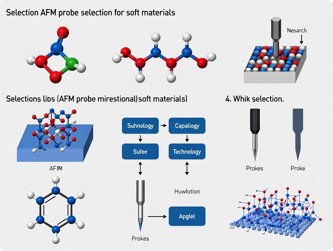
Choosing the Right AFM Probe: The Ultimate Guide for Soft Materials in Biomedical Research

Abstract

This comprehensive guide addresses the critical challenge of Atomic Force Microscopy (AFM) probe selection for characterizing soft biological materials. Tailored for researchers, scientists, and drug development professionals, it moves from foundational principles and probe mechanics to practical methodologies for cell mechanics, polymers, and hydrogels. The article provides actionable troubleshooting for common issues like sample damage and artifacts, offers a comparative analysis of probe types for specific applications, and concludes with validation strategies and future implications for clinical and pharmaceutical research.

Understanding AFM Probe Mechanics: The Foundation for Soft Material Analysis

Troubleshooting Guides & FAQs

Q1: My AFM cantilever "sticks" to my hydrogel sample, often jumping into contact. What is the cause and how can I resolve it? A: This is a classic meniscus force issue caused by a thick fluid layer on the hydrated sample. The water layer creates a strong capillary bridge between the probe and sample.

• Solution Checklist:
  • Use a Sharper, More Hydrophobic Probe: Switch to a silicon nitride (SiN) probe with a sharper tip geometry (e.g., DNP or SNL series). The hydrophobic nature reduces water adhesion. For ultimate reduction, use a carbon-coated tip.
  • Reduce Environmental Humidity: Perform imaging in a sealed fluid cell or a glove box with controlled, lower humidity if not fully immersed.
  • Adjust Engagement Parameters: In your AFM software, significantly reduce the engage "setpoint" (force threshold) and engage velocity.
  • Ensure Full Immersion: For true hydrated samples, complete immersion in buffer is often the most reliable method to eliminate meniscus forces entirely.

Q2: I am getting inconsistent modulus readings from my live cell measurements. Why does the data vary so much? A: Inconsistency often stems from probe wear, inappropriate model choice, or sample viscoelasticity.

• Troubleshooting Steps:
  • Probe Calibration & Wear: Calibrate the spring constant (k) of your cantilever in fluid before each experiment. Visually inspect the tip before and after via SEM if possible; blunt tips overestimate modulus.
  • Model Selection: Ensure you are using a contact mechanics model appropriate for your tip shape and sample (e.g., Hertz, Sneddon, Derjaguin–Muller–Toporov (DMT)). For soft samples, the DMT model often corrects for adhesion.
  • Speed Dependence: Hydrated biological samples are viscoelastic. Perform force curves at multiple approach/retract speeds to characterize and account for this rate-dependent response. Use a table to record modulus vs. speed.

Q3: The probe seems to be dragging or deforming the sample surface during imaging instead of tracing its true topography. A: This indicates excessive lateral forces, often due to a stiff probe or high loading force.

• Resolution Protocol:
  • Switch to a Softer Cantilever: Use a probe with a spring constant (k) closely matched to the sample stiffness. For most cells and hydrogels, aim for k between 0.01 and 0.5 N/m.
  • Employ a Gentler Mode: Transition from Contact Mode to a dynamic (oscillatory) mode like Tapping Mode (in air) or Quantitative Imaging (QI) / PeakForce Tapping (in fluid). These modes minimize lateral shear forces.
  • Optimize Imaging Parameters: Reduce the setpoint/amplitude, and increase the oscillation frequency to minimize sample interaction time.

Table 1: Common AFM Probe Types for Soft, Hydrated Samples

Probe Material	Typical Spring Constant (k) Range	Tip Geometry (Nominal)	Best For	Key Limitation
Silicon Nitride (SiN)	0.01 - 0.6 N/m	Pyramidal, ~20nm radius	Live cells, hydrogels, adhesion force mapping	Moderate wear in fluid; can have high adhesion.
Silicon (Si) with Coating	0.1 - 40 N/m	Sharp spike, conical, ~2-10nm radius	High-res imaging of fixed cells, protein structures	Very stiff unless ultra-low-k levers used; prone to wear.
Carbon-Coated Si or SiN	0.02 - 2 N/m	Same as base, coating adds ~10nm	Combined electrical & mechanical mapping, reduced adhesion	Coating can wear, altering properties over time.
Colloidal Probe (Sphere)	0.1 - 5 N/m	Spherical, 1-10µm diameter	Bulk modulus, adhesion studies, no substrate damage	Low lateral/topographical resolution.

Table 2: Effect of Imaging Mode on Sample Interaction Forces

Imaging Mode	Typical Force Applied	Lateral Shear Forces	Hydrated Sample Suitability	Key Parameter to Optimize
Contact Mode	High (nN to µN)	Very High	Poor (causes deformation/dragging)	Deflection setpoint, scan rate
Tapping Mode (Air)	Medium (pN to nN)	Low	Moderate (for humid, not wet, samples)	Amplitude setpoint, drive frequency
PeakForce QI / Tapping	Low (pN to nN)	Very Low	Excellent (force-controlled)	Peak Force setpoint, frequency
Force Volume Mapping	Variable (user-defined)	None during approach	Good (slow, quantitative)	Max force, trigger threshold, point density

Experimental Protocol: Measuring Viscoelasticity of a Hydrogel

Objective: To map the elastic modulus and relaxation time of a polyacrylamide hydrogel using force spectroscopy. Materials: See "Scientist's Toolkit" below. Procedure:

• Sample Preparation: Prepare a ~100 µm thick polyacrylamide gel of known concentration on a glass-bottom Petri dish. Incubate in PBS for 1 hour before measurement.
• Probe Selection & Calibration: Mount a soft SiN cantilever (k ≈ 0.06 N/m). Calibrate the spring constant using the thermal tune method in PBS.
• AFM Setup: Engage the probe with the sample fully immersed in PBS. Use a force mapping or QI mode.
• Force Curve Programming: Define a grid (e.g., 32x32 points). For each point, program a force curve with:
  • Approach velocity: 2 µm/s.
  • Trigger threshold: 500 pN (to limit indentation).
  • Dwell time at maximum load: 1 second (critical for relaxation measurement).
• Data Acquisition: Acquire the map over a representative area (e.g., 20 µm x 20 µm).
• Analysis:
  • Elastic Modulus: Fit the approach curve segment using the Hertz/Sneddon model for a pyramidal tip.
  • Relaxation Time: Fit the force decay during the dwell segment to a standard linear solid (SLS) or power-law model to extract characteristic relaxation time (τ).

Diagrams

Title: Probe Selection Workflow for Soft Samples

Title: Meniscus Force & Sample Deformation Problem

The Scientist's Toolkit: Essential Materials for Soft Sample AFM

Item	Function & Rationale
Soft Silicon Nitride Probes (e.g., Bruker MLCT-Bio)	Low spring constant (0.01 N/m) minimizes sample indentation. Hydrophilic surface reduces capillary forces in fluid.
Liquid AFM Cell	Enables complete sample immersion, eliminating air-fluid meniscus and maintaining physiological conditions.
Poly-L-Lysine or Cell-Tak	Adhesive coating for immobilizing soft samples like lipid vesicles or non-adherent cells onto substrates.
Calibration Gratings (e.g., TGXYZ, PS & HS-PDL)	Verifies lateral (XY) and vertical (Z) scanner accuracy, and tip sharpness pre/post experiment.
PBS (Phosphate Buffered Saline) or Culture Medium	Standard hydration/imaging buffer to maintain sample viability and osmotic balance.
Spring Constant Calibration Kit (e.g., thermal tune standard)	Essential for accurate in-situ force calibration, as k changes when immersed in fluid.

Welcome to the AFM Probe Technical Support Center. This resource is designed for researchers, particularly those in soft materials and drug development, navigating probe selection and troubleshooting within the context of soft materials research.

Troubleshooting Guides & FAQs

Q1: My AFM images of a hydrogel sample appear overly distorted and “smeared.” The measured modulus seems too high. What could be wrong? A: This is a classic sign of excessive probe-sample force, often due to an inappropriate spring constant. For soft materials, the probe stiffness can dominate the measurement. Use a probe with a lower spring constant (e.g., 0.1 N/m instead of 40 N/m) to minimize indentation and deformation. Ensure you have calibrated the spring constant recently using the thermal tune method.

Q2: I cannot achieve a stable oscillation in tapping mode on my live cell sample. The amplitude phase is noisy. A: Instability in liquid is frequently related to the resonance frequency and coating. The probe’s resonant frequency in air drops significantly in fluid. First, select a probe with a lower nominal resonance frequency (e.g., 20-65 kHz) designed for liquid use. Second, ensure the probe coating is appropriate; a hydrophilic coating (e.g., SiO₂) improves performance in aqueous environments by reducing meniscus forces. Adjust the drive frequency to the new, lower in-liquid resonance peak.

Q3: My high-resolution scan of protein aggregates lacks expected detail. The features look blunt. A: This points to tip geometry wear or contamination. High-aspect-ratio features require a sharp tip. You may be using a standard silicon nitride tip (radius ~20 nm) which is too blunt. Switch to an ultra-sharp silicon tip (radius < 10 nm) or a dedicated high-aspect-ratio tip. Regularly inspect tips via SEM or perform tip-characterization scans using a known sample like TGT1 grating.

Q4: When switching from imaging in air to buffer, my deflection sensitivity changes drastically. Are my force curves invalid? A: Yes, if uncorrected. The laser’s path through liquid bends differently. You must recalibrate the deflection sensitivity in the same medium you will perform measurements. Before your experiment in liquid, capture a new force curve on a clean, rigid substrate (e.g., glass or sapphire) submerged in your buffer to obtain the correct sensitivity value.

Q5: I see significant drift in my force spectroscopy measurements on a lipid bilayer over time. A: Thermal drift is a common challenge. Use a probe with a higher resonance frequency. A higher f₀ often correlates with a smaller cantilever, which has a faster thermal response time and lower drift. Allow the system to thermally equilibrate for at least 30-60 minutes after introducing the liquid cell. Consider using a temperature stabilization stage if available.

Quantitative Parameter Comparison Table

Parameter	Typical Range for Soft Materials	Recommended for Very Soft Samples (e.g., Cells, Hydrogels)	Recommended for Medium Stiffness (e.g., Polymers, Bilayers)	Key Impact on Experiment
Spring Constant (k)	0.01 - 2 N/m	0.01 - 0.1 N/m	0.1 - 0.6 N/m	Determines indentation depth & force control. Too high damages sample; too low reduces stability.
Resonance Frequency (f₀) in Air	10 - 150 kHz	10 - 65 kHz (for liquid use)	65 - 150 kHz	Affects imaging speed & sensitivity to viscosity. Lower f₀ is better for liquid environments.
Tip Radius (R)	< 10 nm (Sharp) to > 50 nm (Standard)	10 - 30 nm (for gentle contact)	< 10 nm (for high-res)	Defines lateral resolution. Sharper tips resolve finer features but wear faster.
Coating	Uncoated Si₃N₄, Si, Au, SiO₂	Hydrophilic SiO₂ (for liquid)	Reflective Au/Al (for laser)	Influences reflectivity, Q-factor, and chemical interactions (e.g., hydrophilicity).

Experimental Protocols

Protocol 1: Thermal Tune Method for Spring Constant Calibration

This method is essential for accurate quantitative force measurements.

• Isolate the cantilever from external vibrations and ensure it is not in contact with any surface.
• In the AFM software, activate the thermal tune function. The system will record the cantilever's thermal fluctuation spectrum.
• Fit the recorded power spectral density (PSD) to a simple harmonic oscillator model. The software will automatically calculate the area under the peak.
• The spring constant k is derived using the Equipartition Theorem: k = k_B T / , where k_B is Boltzmann's constant, T is temperature, and is the mean squared deflection. The software requires the calibrated deflection sensitivity input to complete this calculation.
• Repeat 3-5 times and average the result for accuracy.

Protocol 2: Deflection Sensitivity Calibration in Liquid

Crucial for all force spectroscopy in fluid.

• Submerge your probe and a clean, rigid substrate (e.g., freshly cleaved mica or glass) in your experimental buffer.
• Approach the surface and obtain a force-distance curve using a high trigger threshold (e.g., 5-10 V) to ensure a hard contact.
• On the retract curve, identify the linear region where the tip is in constant, rigid contact with the substrate (slope ≠ 0).
• Fit a straight line to this linear portion. The inverse of this slope (in nm/V) is your deflection sensitivity. Note: This value is medium-dependent and must be measured fresh for each session/medium.

Visualizing Probe Selection Logic

Title: AFM Probe Selection Logic for Soft Materials

The Scientist's Toolkit: Research Reagent Solutions

Item	Function in Soft Materials AFM
Silicon Nitride Probes (Uncoated)	Standard for contact mode in liquid. Biocompatible, low stiffness (0.06-0.6 N/m), suitable for cells and biomolecules.
Sharp Silicon Probes (PPP-NCHR)	High-resolution tapping mode in air. Very sharp tip (<10 nm) for imaging nanostructures on polymer surfaces.
Hydrophilic SiO₂ Coated Probes	Reduces meniscus/adhesion forces in aqueous environments, crucial for stable imaging of soft, wet samples.
Calibration Gratings (TGT1, PG)	Used for scanner calibration and tip characterization. Assess tip wear and shape by imaging sharp spike structures.
Cleaved Mica Disks	An atomically flat, negatively charged substrate for adsorbing proteins, lipid bilayers, or polymers for imaging.
Sapphire or Glass Substrates	Provides an ultra-rigid, inert surface for accurate deflection sensitivity calibration in liquid.
PBS or Appropriate Buffer	Maintains physiological or controlled chemical conditions for biological samples during liquid imaging/FS.
Cantilever UV Cleaning Chamber	Removes organic contaminants from probe surfaces prior to use, improving consistency and reducing adhesion.

Technical Support Center: Troubleshooting & FAQs

This support center is designed for researchers selecting and using Atomic Force Microscopy (AFM) probes for soft materials research, such as biological samples, hydrogels, and polymers. The choice between Silicon (Si), Silicon Nitride (SiN), and Novel Polymer probes is critical for data fidelity and sample integrity.

Frequently Asked Questions (FAQs)

Q1: My AFM images of a live cell membrane show streaks and apparent damage. I'm using a standard silicon probe. What is the likely cause and solution? A: The likely cause is excessive force from the stiff Si probe (spring constant ~0.1-70 N/m) plowing through or indenting the soft cell surface. Switch to a softer probe. Use a SiN cantilever (spring constant ~0.01-0.06 N/m) for contact mode or a "soft" Si probe (~0.1-0.7 N/m) with a polymer tip for tapping mode. Always perform a force calibration before imaging and minimize the setpoint.

Q2: When scanning a novel hydrogel in fluid, my images are featureless and lack contrast. I am using a SiN probe. What should I check? A: This often indicates probe contamination or adhesion. In fluid, hydrophobic contaminants or a sticky sample can cause meniscus forces. First, perform rigorous UV-ozone or plasma cleaning of the probe. If the issue persists, switch to a sharper, hydrophilic probe. Consider a novel polymer probe (e.g., PEG-coated) designed to minimize adhesion in aqueous environments. Ensure your fluid cell is clean and free of bubbles.

Q3: The resonance frequency and quality factor (Q) of my new probe in air do not match the vendor specifications. Is the probe defective? A: Not necessarily. First, recalibrate the sensitivity on a clean, hard sample (e.g., sapphire). Environmental factors like humidity and temperature significantly affect Q and, to a lesser extent, resonance frequency. Ensure the lab environment is stable. If discrepancies remain >15%, the thermal tune method may reveal a damaged or contaminated cantilever. Compare with another probe from the same wafer/box.

Q4: I need to functionalize my probe with a specific ligand for force spectroscopy on proteins. Which probe material is most suitable? A: Silicon Nitride is the traditional choice due to its native hydroxyl groups, which facilitate silane chemistry for covalent attachment. However, novel polymer probes offer superior options. Probes with gold coatings allow for thiol-based chemistry, while carboxylated or amine-functionalized polymer tips provide direct coupling sites via EDC/NHS chemistry. Select based on your specific coupling protocol and required tip geometry.

Q5: The sharp tip of my silicon probe appears to have broken off after contact with a hard contaminant on my polymer sample. How can I prevent this? A: Silicon tips are brittle. Always perform an initial low-resolution scan to identify hard contaminants or sample edges. Use engaging setpoints as low as possible. For heterogeneous samples with unknown hardness, consider using a diamond-coated Si probe for extreme durability or a polymer-based probe, which can be more compliant and resistant to fracture, though at the cost of ultimate sharpness.

Quantitative Probe Data Comparison

Table 1: Key Mechanical and Physical Properties of AFM Probe Materials

Property	Silicon (Si)	Silicon Nitride (SiN)	Novel Polymers (e.g., Polyimide, PEG-based)
Typical Spring Constant (N/m)	0.1 - 70	0.01 - 0.1	0.001 - 0.5
Resonance Freq. in Air (kHz)	10 - 300	5 - 60	1 - 30
Tip Radius (nominal)	<10 nm	20 - 60 nm	20 - 100+ nm
Young's Modulus (GPa)	~130-180	~290	0.001 - 5
Best For	Hard materials, high-res imaging, tapping mode	Soft contact mode, bio-cells in fluid, force spectroscopy	Ultra-soft materials, minimal adhesion, in situ functionalization
Key Limitation	Brittle, high adhesion in fluid	Blunter tip, hygroscopic	Lower durability, limited max temp

Table 2: Troubleshooting Guide: Symptoms and Probable Causes

Observed Problem	Probable Cause (Probe-Related)	Recommended Action
Streaking, sample deformation	Excessive force (too stiff a probe)	Switch to lower spring constant probe (SiN or soft polymer).
Poor resolution, blurred features	Contaminated or broken tip	Clean probe (UV/Ozone); image test grid; replace probe.
Irreproducible force curves	Hydrophobic contamination or sticky tip	Clean probe; use hydrophilic-coated probe (e.g., polymer).
Drifting thermal tune spectra	Environmental instability or loose probe	Stabilize temperature/humidity; re-mount probe.
No signal or erratic deflection	Misaligned laser or damaged cantilever	Realign laser on cantilever; replace probe.

Experimental Protocols

Protocol 1: Calibration of Cantilever Spring Constant via Thermal Tune Method

• Objective: To determine the accurate spring constant (k) of an AFM cantilever in its operating environment.
• Materials: AFM with thermal tune software, clean, vibration-isolated environment.
• Procedure:
  • Mount the probe securely in the holder.
  • Position the probe in the operational configuration (e.g., in air or fluid) without engaging the sample.
  • Acquire the thermal fluctuation spectrum of the cantilever over a sufficient bandwidth (typically 0-1 MHz).
  • Fit the fundamental resonance peak to a simple harmonic oscillator model.
  • The software calculates k using the equipartition theorem: k = k_B * T / <z^2>, where k_B is Boltzmann's constant, T is temperature, and <z^2> is the mean-squared deflection.
• Note: This method is sensitive to environmental noise. Perform multiple times and average.

Protocol 2: Functionalization of a Silicon Nitride Probe for Ligand Binding Studies

• Objective: To covalently attach a specific amine-containing ligand to a SiN tip surface.
• Materials: SiN probe, ethanol, (3-Aminopropyl)triethoxysilane (APTES), glutaraldehyde, ligand of interest, phosphate buffer saline (PBS).
• Procedure:
  • Cleaning: Treat the probe with oxygen plasma for 2-5 minutes to generate hydroxyl groups.
  • Silanization: Vapor-phase or solution-phase incubation with APTES (e.g., 5% in toluene) for 1 hour, followed by curing at 110°C for 10 min. Rinse with toluene and ethanol.
  • Cross-linking: Incubate the probe in a 2.5% glutaraldehyde solution in PBS for 30 minutes. Rinse thoroughly with PBS.
  • Ligand Coupling: Immerse the tip in a solution containing your amine-bearing ligand (e.g., protein, peptide) for 1 hour at room temperature.
  • Quenching & Storage: Quench unreacted aldehyde groups with 1M ethanolamine (pH 8.5) for 10 min. Rinse with PBS and use immediately or store in PBS at 4°C.

The Scientist's Toolkit: Research Reagent Solutions

Table 3: Essential Materials for AFM Probe-Based Soft Materials Research

Item	Function	Example/Notes
APTES	Silane coupling agent for functionalizing Si/SiN surfaces.	Creates an amine-terminated surface for further chemistry.
Sulfo-SMCC	Heterobifunctional crosslinker for linking amines to thiols.	Useful for attaching specific proteins to gold-coated probes.
PEG Spacers	Polyethylene glycol chains minimize non-specific adhesion.	Critical for single-molecule force spectroscopy.
BSA	Bovine Serum Albumin.	Used as a blocking agent to passivate surfaces and probes.
Mica Substrate	Atomically flat, negatively charged surface.	Ideal for preparing lipid bilayers or adsorbing biomolecules.
UV/Ozone Cleaner	Removes organic contaminants from probe surfaces.	Essential step before probe functionalization or high-res imaging.

Visualizations

Decision Tree for AFM Probe Selection on Soft Materials

Probe Functionalization Workflow for Force Spectroscopy

Technical Support Center

Troubleshooting Guides & FAQs

Q1: My AFM images of a hydrogel sample in Contact Mode show severe deformation and tearing. What is the cause and how can I resolve it? A: This is a classic issue with soft materials in Contact Mode. The cause is excessive lateral (shear) forces applied by the scanning tip, which distorts or damages the sample. To resolve:

• Switch to a dynamic mode: Immediately transition to Tapping Mode or, preferably, PeakForce Tapping mode to eliminate lateral shear forces.
• Reduce applied force: If you must use Contact Mode, drastically reduce the setpoint. Use the minimum force required for deflection feedback.
• Use a softer cantilever: Select a cantilever with a spring constant (k) < 0.1 N/m. See the "Probe Selection Table" below.
• Verify calibration: Ensure your cantilever sensitivity and spring constant are accurately calibrated.

Q2: In Tapping Mode, my adhesion measurements on lipid bilayers are inconsistent and the phase signal is unstable. What should I check? A: Inconsistent data in Tapping Mode often stems from inappropriate probe choice or environmental factors.

• Probe resonance: Ensure you are tapping at the true fundamental resonance frequency. Perform a thermal tune in fluid.
• Amplitude ratio: For soft samples, use a free amplitude (A0) of 10-20 nm and a setpoint ratio (Asp/A0) > 0.8 to minimize tip-sample interaction force.
• Probe contamination: A contaminated tip causes unstable oscillation. Clean the tip and cantilever using UV-ozone or plasma cleaning before use.
• Environmental control: For lipid bilayers, ensure temperature stability and that the buffer is free of bubbles.

Q3: When using PeakForce Tapping on live cells, the quantitative modulus values seem too high compared to literature. How do I validate my setup? A: Inaccurate modulus values typically arise from incorrect probe parameters or analysis settings.

• Probe spring constant: This is the most critical parameter. Use the thermal tune method in the same medium (e.g., cell culture medium) as your experiment to measure 'k' accurately.
• Tip radius calibration: Use a known calibration sample (e.g., TiO2 nanoparticles or a grating) to characterize the tip radius before and after experiments. An enlarged radius will overestimate modulus.
• Fit model & range: Use the appropriate contact model (e.g., DMT or Sneddon) for your sample. Ensure the fit is applied only to the suitable portion of the retraction curve. See the "Experimental Protocol" section.
• Trigger force: Use the lowest possible PeakForce Setpoint that provides a stable image (typically 50-150 pN for cells).

Data Presentation: AFM Probe Selection Guide for Soft Matter

Table 1: Mode Comparison & Optimal Probe Parameters for Soft Materials

Mode	Typical Spring Constant (k)	Typical Frequency (f₀)	Optimal Tip Radius	Key Advantage	Primary Challenge
Contact Mode	0.01 - 0.1 N/m	N/A (Static)	20-60 nm	High scan speed, direct force control.	High lateral shear forces damage soft samples.
Tapping Mode	1 - 40 N/m (in air) 0.1 - 1 N/m (in fluid)	70-400 kHz (in air) 10-60 kHz (in fluid)	5-10 nm (sharp)	Eliminates lateral forces, good for topography.	Indirect force control; complex tip-sample dynamics.
PeakForce Tapping	0.1 - 0.7 N/m	1-150 kHz (tuning freq.)	2-60 nm (varies by app.)	Direct, quantitative force control at kHz rates; simultaneous mapping of multiple properties.	Requires precise calibration of k and tip radius.

Table 2: Recommended Probe Types for Common Soft Materials

Sample Type	Recommended Mode	Specific Probe Recommendation	Rationale
Live Mammalian Cells	PeakForce Tapping	Bruker SCANASYST-FLUID+ (k ~0.7 N/m)	Optimized geometry for cell imaging; provides nanoscale modulus mapping in fluid.
Lipid Bilayers & Vesicles	Tapping Mode (in fluid)	Bruker SNL (k ~0.06-0.35 N/m)	Ultra-sharp silicon nitride tip for high resolution; low spring constant minimizes indentation.
Synthetic Hydrogels	PeakForce Tapping	Bruker RTESPA-150 (k~6 N/m) or SCANASYST-AIR (k ~0.4 N/m)	Stiffer probe for deeper modulus analysis of thicker gels or softer probe for surface mapping.
Polymers (thin film)	Tapping Mode (in air)	NanoWorld PointProbe NCHR (k ~42 N/m)	High resonance frequency for stable oscillation and high-resolution surface topography.
Single Protein/DNA	Contact or PeakForce Tapping	Olympus Biolever Mini (k ~0.03 N/m)	Extremely low noise and soft spring constant for piconewton-level force detection.

Experimental Protocols

Protocol 1: PeakForce Tapping Nanomechanical Mapping of Live Cells

• Probe Preparation: Calibrate the spring constant (k) of a SCANASYST-FLUID+ probe using the thermal tune method in complete cell culture medium at experimental temperature.
• Sample Mounting: Plate cells on a 35 mm Petri dish. Before imaging, replace medium with fresh, pre-warmed, CO₂-independent medium to minimize pH drift.
• Microscope Setup: Mount dish on the AFM stage equipped with a fluid cell and temperature controller (set to 37°C).
• Engagement: Use the optical microscope to position the tip above a cell periphery. Engage in PeakForce Tapping mode with a low PeakForce Setpoint (~100 pN).
• Imaging Parameters: Set a scan rate of 0.5-1 Hz with 256-512 samples/line. Adjust the PeakForce Frequency (typically 1-2 kHz) for optimal sample tracking.
• Data Acquisition: Capture simultaneous height, PeakForce Error, DMT Modulus, and Adhesion maps. Apply a live plane fit to the height channel.
• Post-processing: Use analysis software to apply a modulus fit model (e.g., DMT) to the force curves, using a Poisson's ratio assumption of 0.5 for cells.

Protocol 2: High-Resolution Tapping Mode Imaging of Lipid Bilayers

• Probe Preparation: Clean an SNL probe via UV-ozone treatment for 10 minutes. Perform thermal tune calibration in the imaging buffer (e.g., PBS or HEPES).
• Bilayer Preparation: Prepare a supported lipid bilayer on a freshly cleaved mica substrate via vesicle fusion.
• Engagement: Inject buffer into the fluid cell. Engage in fluid, away from the bilayer surface, using a low drive amplitude and a setpoint ratio (rsp) > 0.9.
• Optimization: Tune to the fundamental resonance peak. Adjust the drive amplitude to achieve a free oscillation amplitude (A0) of 5-10 nm.
• Imaging: Scan at 2-4 Hz with 512 samples/line. Continuously adjust the setpoint to maintain a low, constant phase lag.

Mandatory Visualization

Title: Decision Workflow for Selecting AFM Mode on Soft Matter

Title: PeakForce Tapping Operational Cycle & Data Acquisition

The Scientist's Toolkit: Research Reagent Solutions

Table 3: Essential Materials for Soft Matter AFM Experiments

Item	Function/Description	Example Product/Brand
Ultra-Sharp AFM Probes	For high-resolution imaging of biomolecules and fine structures. Tip radius < 10 nm.	NanoWorld SSS-NCHR, Bruker SNL
Soft Bio-Levers	Cantilevers with very low spring constant (k ~0.01-0.1 N/m) for minimal force on delicate samples.	Olympus (now Bruker) BL-AC40TS
PeakForce Tapping Probes	Probes optimized for quantitative nanomechanical mapping with controlled tip geometry.	Bruker SCANASYST series
Calibration Samples	Grids or particles with known dimensions for verifying scanner and tip radius accuracy.	Bruker TGXYZ, Ted Pella Au nanoparticles
Freshly Cleaved Mica	An atomically flat, negatively charged substrate for preparing lipid bilayers or adsorbing biomolecules.	Ted Pella Mica Discs, Grade V-4
UV-Ozone Cleaner	Removes organic contaminants from AFM probes and substrates to ensure clean interactions.	Novascan PSD Series
Temperature Controller	Maintains physiological or controlled temperature for live-cell or polymer studies.	Bruker BioHeater
CO₂-Independent Medium	Prevents pH drift during long-term live-cell imaging in open fluid cells.	Gibco Leibovitz's L-15 Medium
Sylgard 184 PDMS	Elastomer used for making soft calibration samples or as a compliant substrate for cells.	Dow Silicones
BSA (Bovine Serum Albumin)	Used to passivate AFM tips and fluid cells to reduce non-specific adhesion.	Sigma-Aldrich A7906

Technical Support Center: AFM Probe Selection for Soft Materials

Troubleshooting Guide & FAQs

Q1: My AFM cantilever is sticking to or damaging my hydrogel sample. How do I select a probe to avoid this?

A: This indicates excessive adhesion or force. For hydrogels (Young’s modulus ~0.1 kPa to 100 kPa), use a probe with:

• Low Spring Constant: 0.01 - 0.1 N/m to prevent indentation damage.
• Large Tip Radius: >20 nm spherical (colloidal) probes to distribute stress.
• Hydrophilic Coating: Silicon Nitride (SiN) or PEG-modified tips to minimize adhesive capillary forces.
• Protocol: Perform a force curve on a glass slide first to calibrate the exact spring constant using the thermal tune method. Then, approach the hydrogel in fluid (PBS) to eliminate air-liquid meniscus forces.

Q2: When imaging live cells, I get noisy, inconsistent data. What is the optimal probe and mode?

A: Live cells are viscoelastic and dynamic. Use:

• Probe Type: Silicon nitride (SiN) tipless cantilevers with attached microsphere (5-10 µm diameter) for low stress.
• Spring Constant: 0.01 - 0.06 N/m.
• AFM Mode: Use Quantitative Imaging (QI) or Force Mapping mode, not contact mode. This minimizes lateral shear forces.
• Protocol: Conduct experiments in CO₂-independent medium at 37°C. Allow cells to equilibrate for 30 min after transferring to the AFM stage. Set a trigger force ≤ 100 pN and a low approach/retract speed (1-5 µm/s).

Q3: My measurements on lipid bilayers are unstable and seem to penetrate the membrane.

A: Lipid bilayers are extremely soft (<10 MPa) and fluid. Configuration is key.

• Probe: Use a sharp, unused silicon probe with a medium spring constant (~0.1-0.2 N/m) for precise positioning.
• Functionalization: Tip should be hydrophilic (plasma clean) or specifically functionalized (e.g., with cholesterol) to interact with the bilayer headgroups, not penetrate.
• Protocol: Perform imaging in force spectroscopy mode. Use a very small trigger force (50 pN). Ensure bilayers are supported on a smooth mica substrate in an appropriate buffer (e.g., HEPES with Ca²⁺ for supported bilayers).

Q4: How do I choose between a sharp tip and a colloidal probe for tissue sections?

A: It depends on the desired resolution vs. representative modulus.

• Sharp Tip (nominal radius <10 nm): For high-resolution mapping of heterogeneous tissue components (e.g., collagen fibers vs. matrix). Use a soft cantilever (0.1-0.3 N/m). Risk: over-indentation on very soft areas.
• Colloidal Probe (radius 1-10 µm): For measuring bulk, averaged mechanical properties of a tissue region. Better for reproducible elastic modulus measurement.
• Protocol: For fixed tissue sections, ensure they are hydrated in buffer. Map a large area with the colloidal probe first, then target specific structures with a sharp tip.

Q5: My force curves on soft materials show a large hysteresis between approach and retract. Is this an error?

A: Not necessarily. Hysteresis often indicates viscoelasticity or adhesion, which are material properties of soft samples.

• Action: Analyze approach and retract curves separately.
  • Approach Curve Fit: Use Hertz/Sneddon model for elastic modulus.
  • Retract Curve Analysis: Look for adhesive events (e.g., polymer chain unbinding, membrane tether formation).
• Probe Selection: To quantify adhesion, use a probe with a well-defined geometry (colloidal sphere) and a consistent surface chemistry.

Table 1: Recommended AFM Probe Parameters for Soft Material Classes

Material Class	Approx. Young's Modulus	Recommended Spring Constant	Ideal Tip Geometry	Key Mode & Environmental Consideration
Lipid Bilayers	1 - 100 MPa	0.05 - 0.2 N/m	Sharp (R<20nm) or FluidFM	Force Spectroscopy; Liquid, supported substrate
Live Mammalian Cells	0.5 - 100 kPa	0.01 - 0.06 N/m	Colloidal Sphere (R=2.5-10µm)	QI/Force Mapping; Liquid, 37°C, physiological buffer
Hydrogels (e.g., PA, Alginate)	0.1 - 100 kPa	0.01 - 0.1 N/m	Large Colloid (R>20µm)	Force Mapping; Liquid to prevent drying
Fixed Tissue Sections	1 kPa - 1 GPa (heterogeneous)	0.1 - 0.5 N/m	Sharp (R<10nm) or Colloid	Force Mapping; Hydrated buffer
Polymers (e.g., PDMS)	1 MPa - 3 GPa	0.2 - 2 N/m	Sharp or Cube Corner	Contact Mode or QI; Ambient or liquid

Table 2: Common Force Curve Artifacts and Solutions

Artifact	Likely Cause	Probable Probe Issue	Solution
No Detachment	Excessive adhesion, tip sticking	Contaminated/hydrophobic tip	Plasma clean tip; use liquid environment; reduce dwell time.
Irregular Baseline	Drift, thermal fluctuations	Improper thermal calibration	Equilibrate system for 1 hr; recalibrate spring constant in situ.
Sudden Penetration "Pop-in"	Sample rupture or layer break-through	Tip too sharp/stiff for ultra-soft layer	Use softer cantilever, blunter tip; reduce trigger force.
Non-reproducible Slope	Sample creeping/viscoelasticity	Loading rate too high	Reduce approach/retract speed (to 0.1-1 µm/s).

Experimental Protocol: Measuring the Elastic Modulus of a Live Cell Monolayer

Objective: To obtain spatially resolved Young's modulus maps of adherent live cells using AFM.

Materials:

• AFM with environmental chamber and fluid cell.
• Soft colloidal probe (see The Scientist's Toolkit).
• Cell culture medium (without phenol red).
• Confluent cell monolayer on 35 mm petri dish.

Methodology:

• Probe Calibration: Thermal tune the cantilever in air to obtain its spring constant (k). Calibrate the optical lever sensitivity (OLS) on a clean, dry glass slide.
• System Equilibration: Fill fluid cell with warm, CO₂-independent medium. Mount the cell culture dish. Allow 30 minutes for thermal and mechanical drift to stabilize.
• In-situ Sensitivity: Engage on the dish's plastic bottom (a hard, non-deformable area near the cells) to measure the OLS in liquid.
• Mapping Parameters: Set a 10x10 or 20x20 force map grid over a region of interest.
  • Trigger Force: 100-200 pN.
  • Approach/Retract Speed: 2 µm/s.
  • Z-length: 5 µm.
• Data Acquisition: Run the force map. Visually monitor several curves to ensure no damage or excessive indentation (>1 µm).
• Analysis: Fit the approach segment of each force curve (typically 20-80% of the maximum force) with the Hertz/Sneddon model for a spherical indenter to extract the Young's modulus (E). Assume a Poisson's ratio of 0.5 for cells.

The Scientist's Toolkit: Key Research Reagent Solutions

Item	Function in Soft Material AFM
SiN Cantilevers with SiO₂ Microspheres	Gold-standard for soft contact mechanics. The large, defined sphere radius allows accurate Hertz model fitting.
PEG-Linkers for Tip Functionalization	Creates a flexible, bio-inert tether between tip and ligand (e.g., an antibody), enabling specific receptor mapping without non-specific adhesion.
CO₂-Independent Medium (e.g., Leibovitz's L-15)	Maintains pH without a CO₂ incubator during AFM scans, crucial for live-cell experiments.
Plasma Cleaner	Creates a hydrophilic, contaminant-free tip surface, essential for reproducible adhesion measurements and avoiding sample stickiness.
Calcium Chloride (CaCl₂) Solution	Used to promote adhesion and fusion of lipid vesicles to mica for forming supported lipid bilayers (SLBs).
Poly-L-Lysine or Cell-Tak	Used to firmly attach soft samples like tissue sections or hydrogel beads to the substrate for reliable scanning.

Visualizations

Title: AFM Probe Selection Logic for Soft Materials

Title: Live Cell AFM Elasticity Mapping Workflow

Practical AFM Probe Selection Guide for Biomedical Applications

Technical Support Center: Troubleshooting AFM Probe Selection for Live Cell Measurements

Frequently Asked Questions (FAQs)

Q1: My force curves on live cells show excessive indentation (>1 µm) and noisy retraction curves. What is the likely cause and how can I fix it? A1: This typically indicates a probe with excessive stiffness. For live cells (elastic modulus range: 0.1-100 kPa), a cantilever with a spring constant (k) between 0.01-0.1 N/m is recommended. Switch to a softer probe (e.g., silicon nitride tipless cantilever) with a low spring constant. Ensure the thermal tuning method is correctly calibrated in fluid.

• A blocking step (e.g., with 1% BSA for 30 minutes) after conjugating the ligand/biomolecule to the probe.
• Use of a polyethylene glycol (PEG) linker to distance the ligand from the probe surface, reducing steric hindrance.
• Validate functionalization efficacy using a control (e.g., a non-adherent ligand or a bare probe on the same sample).

Q3: My cell elasticity measurements vary dramatically (>50%) between cells of the same type. Is this biological variability or a measurement artifact? A3: While biological variability exists, such high spread often points to instrumental or probe issues. Troubleshoot in this order:

• Probe Contamination: Clean the probe via UV-ozone treatment for 20 minutes before use.
• Loading Rate: Maintain a consistent indentation speed (typically 0.5-2 µm/s). High speeds cause viscoelastic stiffening.
• Indentation Depth: Do not exceed 10% of cell height to avoid substrate effects. Use the "10% rule."
• Temperature & pH: Maintain physiological conditions (37°C, pH 7.4) on the stage top to ensure consistent cell state.

Q4: The probe frequently gets contaminated or damaged during a long experiment. How can I extend probe life? A4: Implement the following protocol:

• Pre-experiment: Use only freshly plasma-cleaned probes.
• During experiment: Engage the probe only when necessary. Retract it fully when moving between points.
• In-line checking: Periodically take force curves on a clean, dry region of the glass substrate to check the probe shape and sensitivity. A sudden change indicates contamination or damage.
• For adhesion mapping: If using a functionalized probe, its effective life is 2-4 hours in buffer. Plan experiments accordingly.

Troubleshooting Guides

Issue: Inconsistent Elasticity Modulus Values

Symptom	Probable Cause	Solution	Verification Step
Values drift upwards over time	Probe contamination by membrane lipids	Clean probe with 2% Hellmanex III solution, rinse with DI water, dry with N2.	Re-measure a calibrated PDMS gel (e.g., 30 kPa). Values should return to baseline.
Sudden drop in measured modulus	Cracked or broken cantilever tip	Replace the probe.	Image the tip using SEM or check optical lever sensitivity (it will be significantly higher).
High point-to-point noise	Low signal-to-noise ratio; probe too stiff	Use a softer cantilever with higher optical lever sensitivity.	Perform thermal tune; the noise floor should be <5 pm/√Hz.

Issue: Poor Adhesion Signal in Force Volume Mapping

Symptom	Probable Cause	Solution	Verification Step
No adhesion peaks detected	Ligand denaturation or incorrect orientation on probe	Optimize functionalization chemistry (e.g., use NHS-EDC for covalent binding, orient with His-tag).	Test probe on a surface coated with the known complementary receptor.
Adhesion force too high, non-specific	Lack of a passivation layer on the probe	Passivate the cantilever with mPEG-SVA or a hydrophilic SAM.	Compare adhesion on a BSA-coated vs. uncoated glass surface; should be minimal.
Adhesion events sporadic	Low ligand density on probe tip	Increase ligand concentration during conjugation.	Use fluorescence microscopy to check ligand density if using fluorescent tags.

Experimental Protocols

Protocol 1: Functionalizing an AFM Probe for Specific Adhesion Mapping Objective: To attach a specific ligand (e.g., an RGD peptide) to a tipless cantilever for mapping integrin adhesion. Materials: Silicon nitride tipless cantilever (k ~ 0.06 N/m), NHS-PEG-Acetylene linker, ligand of interest, copper(II) sulfate, sodium ascorbate, BSA. Steps:

• Clean cantilever in UV-ozone cleaner for 20 min.
• Incubate in 1 mM NHS-PEG-Acetylene solution in DMSO for 1 hour at room temperature.
• Rinse thoroughly in DMSO, then in PBS.
• Prepare a "click chemistry" mix: 100 µM ligand-azide, 1 mM CuSO4, 2 mM sodium ascorbate in PBS.
• Incubate the cantilever in the mix for 30-60 min.
• Rinse in PBS and block in 1% BSA for 30 min.
• Store in PBS at 4°C and use within 8 hours.

Protocol 2: Standardized Live Cell Elasticity Measurement (Force Spectroscopy) Objective: To acquire consistent Young's modulus values from a monolayer of live cells. Materials: AFM with fluid cell, soft colloidal probe (5 µm sphere, k ~ 0.03 N/m), cell culture medium, heated stage. Steps:

• Calibrate the probe's spring constant and sensitivity on a clean glass substrate in medium.
• Maintain sample at 37°C and 5% CO2.
• Select 10-20 cells per condition. On each cell, select 3-5 points away from the nucleus.
• Set force curve parameters: approach speed = 1 µm/s, trigger force = 0.5 nN, retract speed = 1 µm/s.
• For each curve, fit the extending segment using the Hertz/Sneddon model for a spherical tip. Use a Poisson's ratio of 0.5.
• Exclude curves with abnormal approach (e.g., no contact) or retraction (multiple adhesions) features.

Diagrams

Title: AFM Probe Selection Logic for Live Cells

Title: AFM Probe Biofunctionalization Workflow

The Scientist's Toolkit: Research Reagent Solutions

Item	Function & Rationale
Silicon Nitride Tipless Cantilevers (k=0.01-0.1 N/m)	The gold standard for live cell mechanics. Low spring constant prevents cell damage, tipless design allows for precise colloidal probe attachment or direct functionalization.
Colloidal Probes (2-10 µm silica/polystyrene spheres)	Glued to tipless cantilevers to create a well-defined spherical geometry for accurate Hertz model fitting in elasticity measurements.
NHS-PEGn-Acetylene Linkers (e.g., MW: 3400 Da)	Heterobifunctional crosslinkers. NHS ester binds amine on probe surface, PEG spacer reduces non-specific binding, acetylene enables "click" ligand attachment.
Azide-Modified Ligands (Peptides, Antibodies)	Ligand ready for bioorthogonal "click" chemistry conjugation to the PEG linker, ensuring controlled orientation and density.
BSA (Bovine Serum Albumin)	Standard blocking agent to passivate any remaining reactive sites on the functionalized probe, minimizing non-specific adhesion.
Calibrated PDMS/PA Gel Samples (0.1-100 kPa)	Essential reference materials for validating probe performance and ensuring accuracy of modulus measurements before/after cell experiments.
Hellmanex III or SDS Solution (2%)	Effective cleaning agent for removing biological contaminants from probes and AFM fluid cell components.

Imaging and Force Spectroscopy on Proteins and Nucleic Acids

Technical Support Center: Troubleshooting Guides & FAQs

Frequently Asked Questions

Q1: Why is my measured contour length for dsDNA consistently shorter than the expected 0.34 nm per base pair? A: This is a common calibration and sample preparation issue. Expected length is calculated as (number of base pairs * 0.34 nm). Common causes and solutions:

• Sample Adsorption: Incomplete adsorption to the mica surface. Ensure proper divalent cation (e.g., 10 mM NiCl₂ or MgCl₂) treatment for negatively charged mica.
• Stretching Rate: Excessive pulling speed can lead to overstretching before full contour length is achieved. Reduce the retraction velocity to < 1 µm/s.
• Probe Stickiness: A contaminated or overly adhesive tip can detach the molecule prematurely. Use plasma-cleaned, sharp tips (e.g., SNL or MLCT) and ensure buffer is free of organics.

Q2: During force spectroscopy on a multi-domain protein, I see irregular force peaks with inconsistent spacing. What could be wrong? A: Irregular peaks often indicate non-specific adhesion or sample heterogeneity.

• Cause 1: Non-specific interactions between the tip and the protein/substrate. Increase the salt concentration (e.g., 150-300 mM NaCl) in the imaging buffer to screen electrostatic interactions.
• Cause 2: Protein denaturation or aggregation on the surface. Use a fresh, monodisperse sample and a shorter incubation time (< 10 mins).
• Cause 3: Probe selection. A tip that is too blunt or sticky will cause multiple, unspecific attachments. Switch to a non-contact, sharp silicon nitride tip (spring constant ~0.1 N/m) for soft, folded proteins.

Q3: My AFM images of proteins are always blurred with low resolution. How can I improve sharpness? A: Blurred images typically result from poor mechanical stability, tip contamination, or incorrect scanning parameters.

• Protocol Adjustment: Engage at a lower setpoint (reduce amplitude or force). Use a softer cantilever (k ~0.1-0.5 N/m). Optimize scan speed; it should be scaled to scan size (e.g., 1-2 Hz for a 500 nm scan).
• Sample Preparation: Ensure the substrate (e.g., mica) is freshly cleaved. Rinse with buffer thoroughly after sample deposition to remove loosely bound material.
• Environmental Control: Perform imaging in a vibration-isolated enclosure. Allow the fluid cell temperature to equilibrate for 30 minutes to minimize thermal drift.

Q4: When measuring ligand-receptor unbinding forces, my data shows a very wide force distribution. How do I improve precision? A: A wide distribution suggests variability in the linkage chemistry or number of bonds.

• Tip Functionalization: Ensure a consistent, dilute concentration of ligands during tip pegylation. Use a well-established protocol (e.g., PEG-benzaldehyde linker) to provide a long, flexible tether.
• Control Experiments: Always perform blocking experiments with free ligand in solution to confirm specificity.
• Data Analysis: Apply a stringent rupture length filter (based on PEG tether length) to select for single-molecule events. Fit multiple Gaussians to the force histogram to deconvolute single and multiple bond ruptures.

Experimental Protocols

Protocol 1: Imaging Double-Stranded DNA on Mica in Liquid Objective: Achieve high-resolution, reproducible imaging of dsDNA topology.

• Substrate Preparation: Cleave a piece of muscovite mica (Grade V1) using adhesive tape to create a fresh, atomically flat surface.
• Surface Activation: Deposit 50 µL of 10 mM NiCl₂ onto the mica for 2 minutes. Blot dry with filter paper.
• Sample Deposition: Dilute dsDNA (e.g., λ-DNA) in TE buffer (10 mM Tris, 1 mM EDTA, pH 8.0) to ~1 ng/µL. Apply 30 µL to the Ni²⁺-treated mica. Incubate for 3 minutes.
• Rinsing: Gently rinse the surface with 2 mL of the imaging buffer (e.g., 10 mM HEPES, 150 mM KCl, pH 7.5) to remove unbound DNA and salts.
• Imaging: Mount the sample in the fluid cell. Use a sharp, non-contact silicon tip (k = 0.1-0.4 N/m, f₀ ~65 kHz in liquid). Engage in AC mode with a low amplitude setpoint (~0.8 V). Scan at 1-2 Hz with 512x512 resolution.

Protocol 2: Single-Molecule Force Spectroscopy of Protein Unfolding Objective: Measure the unfolding forces of a multi-domain protein (e.g., titin).

• Sample Immobilization: Adsorb the protein (10-50 µg/mL in PBS) onto a freshly cleaved mica surface for 10 minutes. Rinse with PBS to remove excess.
• Tip Functionalization (Optional for specific attachment): Clean cantilever (e.g., MLCT, k=0.1 N/m) in UV-Ozone for 15 mins. Incubate in 1 mM NHS-PEG-Aldehyde linker for 1 hour. Quench with ethanolamine. Incubate with an antibody or specific ligand for the protein terminus.
• Force Curve Acquisition: Approach the surface at 1 µm/s. Upon contact, apply a gentle force (< 100 pN) for 0.5-1 second to allow binding. Retract at a constant velocity of 0.5-1 µm/s.
• Data Collection: Record at least 1000-2000 force-distance curves from different locations.
• Analysis: Use a worm-like chain (WLC) or extended freely jointed chain (FJC) model to fit the sawtooth peaks and extract contour length increments and unfolding forces.

Data Tables

Table 1: Recommended AFM Probes for Soft Biomaterials

Probe Type (Model Example)	Spring Constant (N/m)	Tip Radius	Best For	Key Consideration
Silicon Nitride, Non-Contact (SNL)	0.06 - 0.35	< 10 nm	High-res imaging of proteins/nucleic acids in fluid	Very sharp, minimizes sample deformation.
Silicon, Tapping Mode (AC160)	~26 (in air)	~7 nm	High-speed imaging in air	Stiff; requires lower amplitudes for soft samples.
Gold-coated Silicon (ContAu)	0.01 - 0.6	~20 nm	Force spectroscopy (thiol chemistry)	Easy functionalization, but coatings can degrade.
Nitride Lever, Soft (MLCT)	0.01 - 0.03	~20 nm	Single-molecule unfolding/force-clamp	Ultra-soft for precise force control.
qp-BioAC (SCANASYST-FLUID+)	~0.7	~5 nm	Routine imaging in fluid, high stability	Optimized thermal & mechanical stability.

Table 2: Common Buffers and Additives for Biomolecular AFM

Reagent	Typical Concentration	Function in Experiment
NiCl₂ / MgCl₂	1-20 mM	Divalent cation for anchoring nucleic acids to mica.
HEPES / Tris Buffer	10-50 mM, pH 7.5	Maintains physiological pH and ionic strength.
KCl / NaCl	50-300 mM	Controls ionic strength; screens electrostatic interactions.
PBS	1X	Standard buffer for protein immobilization and activity.
BSA or Casein	0.1-1 mg/mL	Used to passivate surfaces/tips and reduce non-specific binding.
PEG Linkers	1-5 mM	Provides flexible tether for specific single-molecule attachment in force spectroscopy.

The Scientist's Toolkit: Research Reagent Solutions

Item	Function & Explanation
Muscovite Mica (V1 Grade)	Atomically flat, negatively charged substrate. Can be functionalized with cations to adsorb biomolecules.
Nickel(II) Chloride (NiCl₂)	Divalent cation solution. Treats mica to create a positive charge density for strong adsorption of DNA/RNA.
PEG-Based Heterobifunctional Crosslinkers (e.g., NHS-PEG-Aldehyde)	Creates a long, flexible spacer between the AFM tip and biomolecule. Essential for specific, single-molecule force measurements.
BSA (Bovine Serum Albumin)	A common blocking agent. Passivates surfaces and tips to minimize non-specific protein adsorption.
Silicon Nitride Cantilevers (e.g., SNL, BioLever)	Standard probes for liquid imaging. Biocompatible, with a range of soft spring constants suitable for delicate samples.
Piranha Solution (H₂SO₄:H₂O₂)	EXTREME CAUTION. Powerful cleaning agent for silicon-based tips and substrates. Removes organic contaminants.

Diagrams

Diagram 1: AFM Probe Selection Workflow for Soft Materials

Diagram 2: Force Spectroscopy Ligand-Binding Experimental Setup

Technical Support Center: Troubleshooting AFM Analysis of Soft Biomaterials

This technical support center provides guidance for researchers using Atomic Force Microscopy (AFM) to characterize soft synthetic biomaterials, framed within the critical context of AFM probe selection for accurate and reproducible data.

Troubleshooting Guides & FAQs

Q1: My AFM cantilever is sticking to or indenting too deeply into my hydrogel sample, making modulus measurement unreliable. What is the primary cause and solution? A: This is typically caused by excessive loading force due to an overly stiff cantilever. Hydrogels have a Young's modulus in the kPa range. Use a soft cantilever with a spring constant (k) between 0.01 and 0.5 N/m. Always calibrate the spring constant and optical lever sensitivity on a hard surface (e.g., clean silicon) before measuring soft samples. Employ a force mapping mode with a trigger force set below 1-5 nN to prevent sample damage.

Q2: I am imaging a porous polymer scaffold, but the tip seems to get caught in the pores, distorting the topography. How can I improve image fidelity? A: This indicates a tip geometry mismatch. Standard sharp tips (radius ~10nm) can plunge into nanopores. Use a colloidal probe (a microsphere attached to the cantilever, radius 1-10µm) for global topography or a specially etched "whisker" tip with high aspect ratio to reach into pores. Reduce the scan speed and use a non-contact or tapping mode to minimize lateral forces that can drag the tip.

Q3: When measuring the adhesion force of drug carrier nanoparticles, my data shows high variability between particles on the same sample. What should I check? A: High variability often points to tip contamination or heterogeneous sample surface chemistry. First, rigorously clean the tip in UV-Ozone or plasma cleaner before measurements. For the sample, ensure thorough washing to remove unbound surfactants or polymers. Functionally coat your AFM tip with a specific ligand to measure targeted interactions, rather than relying on non-specific silicon nitride tip adhesion. Increase the number of force curves (N>1000) per condition for statistically robust analysis.

Q4: My force spectroscopy curves on a drug-loaded micelle show an unexpected long-range nonlinear region before contact. What does this signify? A: This is likely a measurement artifact from a contaminated liquid environment or the presence of a dynamic polymer brush layer on the micelle. Ensure your buffer is particle-free by using syringe filtration (0.22µm). If studying PEGylated carriers, this nonlinear region could be the actual compression of the hydrated polymer corona. Use an extended fitting model (e.g., Hertz + brush model) instead of the standard Hertz/Sneddon model to quantify both the core modulus and the brush density.

Q5: The modulus I measure for my PDMS standard is significantly different from the known value, calling all my soft material data into question. What is my systematic error? A: The most common error in modulus discrepancy on known standards is incorrect spring constant calibration. Re-calibrate using the thermal tune method in your specific imaging medium (air/water). Secondly, verify your indentation model. For spherical tips, use the Hertz model; for pyramidal tips, use the Sneddon model. Ensure your indentation depth does not exceed 10-15% of the sample thickness to avoid substrate stiffening effects.

Table 1: Recommended AFM Probe Selection for Synthetic Biomaterials

Biomaterial Type	Typical Modulus Range	Recommended Cantilever Spring Constant	Recommended Tip Geometry	Primary AFM Mode
Hydrogel (e.g., Alginate, PEG)	0.1 kPa - 50 kPa	0.01 - 0.1 N/m	Spherical Colloidal Probe (Ø2-10µm)	Force Mapping / QI
Polymer Scaffold (e.g., PCL, PLA)	50 MPa - 2 GPa	1 - 30 N/m	Sharp Silicon Tip (Radius <10nm)	Tapping Mode
Drug Carrier (Micelle/Liposome)	10 MPa - 1 GPa	0.1 - 0.6 N/m	Sharp Silicon Nitride Tip	Force Spectroscopy
Elastic Standard (e.g., PDMS)	1 MPa - 3 MPa	0.1 - 0.5 N/m	Spherical Colloidal Probe (Ø5µm)	Force Spectroscopy

Table 2: Key Parameters for AFM Force Spectroscopy on Drug Carriers

Parameter	Typical Value Range	Impact on Measurement
Trigger Force	0.5 - 2 nN	Prevents sample damage; higher values may induce plasticity.
Approach/Retract Speed	0.5 - 2 µm/s	Affects measured adhesion; slower speeds allow for more molecular interactions.
Dwell Time	0 - 2 seconds	Allows for stress relaxation in viscoelastic materials; critical for accurate modulus.
Curves per Map	256x256 to 512x512	Higher spatial resolution for heterogeneity mapping increases experiment time.

Experimental Protocols

Protocol 1: Measuring the Nanomechanical Properties of a Hydrogel via AFM Force Mapping

• Sample Preparation: Prepare hydrogel on a rigid substrate (e.g., glass slide). For hydrated measurement, create a fluid cell using a silicone O-ring.
• Probe Selection & Calibration: Mount a soft, colloidal probe (k~0.06 N/m). Perform thermal tune calibration in the medium (air or liquid).
• AFM Setup: Engage in contact mode at a very low setpoint (≈0.5V). Switch to the force mapping/quantitative imaging mode.
• Parameter Setting: Set a scan area (e.g., 20x20µm). Define a grid (e.g., 64x64 points). Set trigger force to 1 nN, approach/retract speed to 2 µm/s, and dwell time to 0.1s.
• Data Acquisition: Run the map. The system will acquire a force-distance curve at each pixel.
• Data Analysis: Use the instrument's software to fit the approach curve of each force curve with the Hertz contact model (for spherical tips) to generate spatial maps of Young's modulus and adhesion.

Protocol 2: Probing Ligand-Receptor Binding on a Functionalized Drug Carrier

• Tip Functionalization: Immerse a PEG-linked, biotinylated cantilever in a streptavidin solution (0.1 mg/mL in PBS) for 30 minutes. Rinse gently with PBS.
• Sample Preparation: Deposit drug carrier nanoparticles (e.g., liposomes with biotinylated lipids) on a poly-L-lysine coated mica surface. Rinse to remove unbound particles.
• AFM Setup: Mount the functionalized probe. Engage in liquid (PBS) near a particle using contact mode with minimal force.
• Force Spectroscopy: Position tip over a single particle. Acquire 500-1000 force-distance curves at 1 µm/s with a trigger force of 150 pN.
• Control Experiment: Repeat with a non-functionalized (blocked) tip or add free ligand to solution for competitive inhibition.
• Data Analysis: Plot adhesion force histograms. Specific binding events are identified as discrete unbinding steps in the retract curve and are absent in control experiments.

Diagrams

The Scientist's Toolkit: Research Reagent Solutions

Table 3: Essential Materials for AFM Characterization of Biomaterials

Item	Function	Example Product/Catalog
Soft Cantilevers	For measuring kPa-MPa materials without damage.	Bruker MLCT-Bio-DC (k~0.03 N/m), Olympus RC800PB (k~0.05 N/m)
Colloidal Probes	Spherical tips for well-defined contact on soft, sticky samples.	Novascan PS-QP-SPH (Silica spheres, Ø2-10µm) or custom glue attachment.
Functionalization Kits	For modifying tips with specific chemical/biological groups.	Bruker Peg-LC-Biotin Cantilevers, Nanoscience Instruments SAM Coating Kits.
Calibration Standards	To verify spring constant and modulus measurements.	Bruker PFQNM-LC-Cal (Polystyrene, 2.5 GPa), Asylum Research PDMS Sheets (various moduli).
Sample Substrates	Atomically flat, clean surfaces for sample deposition.	Freshly Cleaved Mica Discs (V1 Grade), Silicon Wafers (P-type).
Syringe Filters	For particle-free buffer preparation in liquid AFM.	PVDF Membrane Filters, 0.22 µm pore size.
UV-Ozone Cleaner	For thorough cleaning of tips and substrates to remove organic contamination.	Novascan PSD Series Digital UV Ozone Cleaner.

Technical Support Center

Troubleshooting Guide

Problem 1: Unstable Baseline and Excessive Noise in Force Measurements

• Potential Cause: Non-specific adsorption of biomolecules (e.g., proteins) onto the probe and cantilever.
• Solution: Implement a rigorous probe cleaning protocol before and after experiments. Use UV-ozone treatment for 20 minutes, followed by rinsing in ethanol and ultrapure water. For biological probes (e.g., PEGylated tips), ensure proper functionalization chemistry to passivate unused reactive sites.
• Preventative Step: Use cantilevers with reflective backside coatings (e.g., Au, Al) optimized for liquid laser reflection. Increase the laser alignment settling time to 30 minutes after introducing liquid to allow for thermal equilibration.

Problem 2: Poor Resonance Peak Detection in Liquid

• Potential Cause: Low quality factor (Q) in liquid damping the thermal tune spectrum.
• Solution: Adjust the thermal tune parameters: Increase the sampling frequency/bandwidth and use a higher number of FFT points (e.g., 8192). Ensure the drive frequency range is appropriately set (typically 5-50% below the in-air resonance frequency for soft cantilevers).
• Alternative Method: Switch to a direct drive (piezo-acoustic) tuning method if available, which provides a stronger excitation signal in viscous media.

Problem 3: Drift in Z-Height and Lateral Position

• Potential Cause: Thermal drift from temperature gradients between the fluid cell, scanner, and environment.
• Solution: Activate the microscope's environmental enclosure and allow the system to equilibrate for at least 1-2 hours with the fluid cell filled. Use a temperature control stage if available. Begin experiments by engaging briefly on a rigid area to calibrate drift rates before moving to the soft sample region.
• Protocol: Perform a drift measurement: Engage on a rigid spot, set a small scan size to zero, and monitor the deflection error signal over 5 minutes. Use the measured drift rate to compensate in software.

Problem 4: Low Imaging Resolution or Tip Contamination

• Potential Cause: Probe damage or a contaminant layer on the tip.
• Solution: Inspect the tip before use via SEM (if possible). In liquid, perform gentle "tapping" on a clean, hard region (e.g., mica) to potentially dislodge soft contaminants. If resolution remains poor, change the probe.
• Critical Check: Verify that the cantilever's spring constant, as calibrated in liquid, is suitable for the sample's modulus. A probe that is too stiff will damage soft samples.

Frequently Asked Questions (FAQs)

Q1: What is the most critical factor when selecting a cantilever for liquid-phase AFM on soft materials? A: The spring constant (k) is paramount. It must be low enough to avoid sample deformation and high enough to overcome adhesive and capillary forces. For most soft biological samples (e.g., cells, hydrogels), a k between 0.01 - 0.1 N/m is ideal. The resonance frequency in liquid should also be considered for dynamic modes.

Q2: How do I accurately calibrate the spring constant of a cantilever in liquid? A: The thermal tune method is standard. Ensure the cantilever is fully immersed and thermally equilibrated. The key is using the correct fluid density and viscosity values for your medium (e.g., water at 25°C: ρ=997 kg/m³, η=0.89 mPa·s). Many AFM software packages have built-in fluid parameters.

Q3: What probe coatings are recommended for biological fluids to reduce noise? A: Reflective gold or aluminum coatings on the cantilever backside are essential for laser reflection. For the tip itself, silicon nitride is inherently hydrophilic and often used. For specific biofunctionalization, a thin chromium/gold coating followed by a PEG linker or other biocompatible monolayer is standard to minimize non-specific binding.

Q4: Can I use the same probe for both imaging and force spectroscopy in liquid? A: It is possible but not always optimal. Sharp, high-aspect-ratio tips (e.g., AC40) are best for high-resolution imaging. For force spectroscopy, tipless cantilevers or those with spherical tips are often preferred to simplify contact geometry and data analysis. Using a dedicated probe for each type of experiment is recommended for rigorous results.

Q5: Why is my force curve "jumpy" or displaying irregular adhesions in buffer? A: This is often indicative of multiple, discrete bond ruptures or the peeling of macromolecular chains. It can be a real signal. To confirm it's not an artifact, ensure your sample and tip are clean, increase the approach/retract velocity to test for rate-dependence, and perform many curves (100+) at different locations to establish reproducibility.

Data Presentation

Table 1: Common AFM Probe Types for Liquid-Phase Soft Material Research

Probe Type	Material	Typical Spring Constant (N/m)	Typical Resonance Freq. in Liquid (kHz)	Best Use Case	Key Consideration in Liquid
MLCT-Bio	Si₃N₄ (Nitride)	0.01 - 0.03	1 - 3	Cell imaging, soft gel mapping	Very soft, susceptible to drift; excellent force sensitivity.
PNP-TR	Silicon	0.08 - 0.6	10 - 30	TREC imaging, molecular recognition	Stiffer, conductive coating needed for most bio-apps.
AC40	Silicon	0.1 - 0.6	15 - 40	High-res imaging of proteins, DNA	Sharp tip; can be functionalized; higher k may deform samples.
qp-Bio	Silicon	0.03 - 0.3	5 - 20	Quantitative force spectroscopy	Four-sided pyramid tip; well-defined geometry for modeling.
Colloidal Probe	Silicon with Sphere	0.1 - 5.0	Varies	Adhesion measurements, single-cell mechanics	Spherical tip simplifies contact mechanics; often custom-made.

Table 2: Troubleshooting Summary: Symptoms, Causes, and Actions

Symptom	Likely Cause	Immediate Action	Long-term Solution
High thermal noise floor	Low Q factor in fluid	Increase FFT points, check laser alignment	Use probes with higher reflective coating; improve fluid cell isolation.
Inconsistent engagement	Surface contamination or electrostatic effects	Clean sample and probe; change buffer ionic strength	Use plasma cleaner for sample/probe; implement better sample prep protocol.
"Double" deflection curve	Tip contamination or multiple contacts	Retract, rinse cell and probe, re-engage	Implement strict cleaning routine; use sharper, cleaner probes.
Cantilever frequency drops suddenly	Biofouling on cantilever arms	Retract immediately, replace probe	Improve probe passivation (e.g., with BSA or PEG solutions).

Experimental Protocols

Protocol 1: In-Situ Spring Constant Calibration via Thermal Tune

• Setup: Mount the probe and fill the fluid cell with the experimental buffer. Align the laser and adjust the photodetector to a sum value of 3-5 V.
• Equilibration: Allow the system to sit for 30 minutes to minimize thermal drift.
• Parameter Setting: Access the thermal tune module. Set the frequency range to 0.5x to 2x the expected in-liquid resonance. Set the FFT points to 8192.
• Acquisition: Acquire the thermal noise spectrum. Fit the fundamental resonance peak to a simple harmonic oscillator model.
• Input Parameters: Enter the precise temperature, fluid density (ρ), and fluid viscosity (η).
• Calculation: The software integrates the power spectral density to calculate the spring constant (k = kB * T / B is Boltzmann's constant, T is temperature, and

Protocol 2: Passivation of Probes for Biofluid Experiments

• Cleaning: Clean a gold-coated cantilever with UV-ozone for 20 minutes.
• Thiol Solution: Prepare a 1 mM ethanolic solution of alkane thiol (e.g., HS-C11-EG₄-OH) for passivation.
• Incubation: Immerse the cantilever in the thiol solution for 18 hours at room temperature in a sealed vial.
• Rinsing: Rinse thoroughly with absolute ethanol and then with the experimental buffer (e.g., PBS).
• Functionalization (Optional): For specific binding, the terminal OH group can be activated for coupling to ligands (e.g., via EDC/NHS chemistry) in a separate step.

Diagrams

Title: AFM Probe Optimization Workflow for Liquid Studies

Title: Root Cause Analysis for High Noise in Liquid AFM

The Scientist's Toolkit: Research Reagent Solutions

Item	Function/Benefit	Key Consideration for Liquid AFM
Silicon Nitride (Si₃N₄) Probes	Biocompatible, hydrophilic surface. Low autofluorescence. Ideal for imaging live cells and biomolecules.	Often have lower spring constants (soft). Susceptible to dissolution in strong bases over time.
Gold-Coated Cantilevers	Provides high laser reflectivity. Surface allows for robust thiol-based chemical functionalization.	Coating can degrade over time in some electrolytic buffers. May increase stiffness slightly.
PEG (Polyethylene Glycol) Linkers	Used to tether ligands to the AFM tip. Provides a flexible spacer, reducing non-specific binding.	Length of PEG chain must be chosen to match the size and accessibility of the target molecule.
BSA (Bovine Serum Albumin)	Common blocking agent to passivate probe and sample surfaces, minimizing non-specific protein adsorption.	Can sometimes form a soft layer that affects very short-range forces. Use at 0.1-1% w/v in buffer.
Functionalization Kits (e.g., EDC/NHS)	Chemistry kits for covalent attachment of amines (e.g., on proteins) to carboxylated surfaces on the tip.	Reactions must be performed in anhydrous or buffered conditions as specified. Efficiency can vary.
Calibration Gratings (e.g., TGZ1, PG)	Standard samples with known pitch and height for verifying lateral and vertical scanner calibration in fluid.	Ensure the grating material is inert in your liquid (e.g., silicon is fine for most aqueous buffers).
UV-Ozone Cleaner	Critical for removing organic contaminants from probes and sample substrates before use or functionalization.	Over-exposure can damage certain coatings. Typical treatment is 15-30 minutes.
Temperature Control Stage	Maintains constant sample temperature, reducing thermal drift and enabling temperature-dependent studies.	Must be compatible with the AFM fluid cell. Check for thermal stability specifications (±0.1°C).

Technical Support Center & FAQs

FAQ: General Probe Selection & Setup Q1: My AFM force curves on a hydrogel show excessive noise and inconsistent indentation. What is the most likely cause and how do I fix it? A1: The most likely cause is using a probe with an inappropriate spring constant or tip geometry. For soft materials (<10 kPa), use a soft cantilever (k ≈ 0.01 - 0.1 N/m) to ensure sufficient sensitivity without excessive indentation. Ensure the tip is clean and free of debris. Perform a thermal tune in fluid prior to measurement to calibrate the spring constant accurately. Use a spherical tip (colloidal probe) if measuring bulk modulus to avoid strain-stiffening artifacts common with sharp tips.

Q2: During a force mapping experiment on live cells, the adhesion force measurements drift over time. How can I stabilize the readings? A2: Drift is often due to thermal instability or sample settling. Allow the system (microscope and fluid cell) to thermally equilibrate for at least 45 minutes after loading. Use a temperature control stage if available. Ensure your buffer is fully degassed to prevent bubble formation under the cantilever. Set a longer pause between measurement points in your mapping grid to allow for fluid stabilization. Consider using a closed-loop scanner to correct for positional drift.

Q3: When performing a stress-relaxation test on a polymer blend, the relaxation curve does not fit standard models. What protocol adjustments should I consider? A3: First, verify your indentation depth is within the linear viscoelastic regime (typically ≤ 10% of sample thickness). Increase the hold phase duration; for many soft materials, relaxation can take tens of seconds. Ensure your approach velocity is consistent and controlled. Switch to a low-stiffness, fluid-damped cantilever designed for dynamic modes to minimize ringing during the fast approach to the hold setpoint.

Q4: The binding specificity in a ligand-receptor binding assay seems low. What controls and calibration steps are mandatory? A4: You must run the following controls: (1) Block the tip with a non-functional ligand or BSA. (2) Measure on a sample area without receptors. (3) Perform the experiment in the presence of a free ligand inhibitor. Calibrate the spring constant daily in the relevant medium. Functionalize tips using a consistent protocol (e.g., PEG spacer of known length) and confirm ligand density via a method like fluorescence labeling if possible.

Table 1: Recommended AFM Probe Parameters for Common Soft Material Assays

Material / Assay	Approx. Modulus Range	Recommended Cantilever Spring Constant	Optimal Tip Geometry	Key Mode / Notes
Hydrogels & ECM Mimics	0.1 - 10 kPa	0.01 - 0.06 N/m	Spherical (2-10µm diameter)	Force Spectroscopy, QI / Use low approach speed (0.5-1 µm/s)
Live Mammalian Cells	0.5 - 20 kPa	0.02 - 0.1 N/m	Pyramidal, sharp (nom. radius < 20nm)	PeakForce QI or Force Volume / Maintain 37°C & CO2
Lipid Bilayers & Vesicles	10 - 200 MPa	0.05 - 0.5 N/m	Sharp pyramidal or bullet-shaped	Force Spectroscopy / Use ultra-low loading rates for pore formation
Polymer Thin Films	1 MPa - 10 GPa	0.1 - 2 N/m	Sharp pyramidal or conical	Nanomechanical Mapping, DART / Control ambient humidity
Protein Fibrils (e.g., Amyloid)	1 - 10 GPa	0.1 - 0.6 N/m	Super-sharp silicon (radius < 10nm)	Torsional Resonance or PeakForce / Scan perpendicular to fibril axis

Detailed Experimental Protocols

Protocol 1: Nanomechanical Mapping of a Synthetic Hydrogel (PeakForce QI)

• Probe & Sample Prep: Mount a soft, spherical colloidal probe (k ~ 0.03 N/m, radius ~5µm). Plasma clean tip for 2 minutes. Prepare hydrogel on a rigid substrate (e.g., glass). Immerse in PBS.
• System Equilibration: Engage the probe in fluid away from the sample. Allow 30 minutes for thermal drift stabilization.
• Calibration: Perform thermal tune in fluid to calibrate spring constant. Adjust deflection sensitivity on a clean, rigid area of the substrate.
• Parameter Setup: Set PeakForce amplitude to 50-100 nm. Set PeakForce frequency to 0.5-1 kHz. Adjust the PeakForce setpoint to achieve ~10-20% sample indentation.
• Mapping & Data Acquisition: Select scan area (e.g., 20x20 µm). Set scan rate to 0.2-0.3 Hz. Acquire map capturing DMT Modulus, Adhesion, and Deformation channels.
• Analysis: Apply plane fit to modulus image. Use histogram tool to determine average modulus, excluding areas of adhesion artifact.

Protocol 2: Single-Molecule Force Spectroscopy for Receptor-Ligand Binding

• Tip Functionalization: Use a silicon nitride tip (k ~ 0.06 N/m). Clean in piranha solution (Caution: Highly corrosive). Incubate in PEG-spacer/linker solution with terminal NHS-ester for 1 hour. Conjugate ligand (e.g., an antibody) to linker by incubation in 50 µg/mL solution for 30 minutes.
• Sample Prep: Immobilize receptor-containing sample (e.g., cell monolayer, supported bilayer) in fluid chamber with appropriate binding buffer.
• Control Measurement: Perform force-distance cycles on a passivated area (blocked with BSA) to establish non-specific adhesion baseline.
• Specificity Test: Move to target area. Set trigger threshold to 10-50 pN. Use approach/retract speed of 400-1000 nm/s. Collect 500-1000 curves per condition.
• Data Processing: Use semi-automated analysis software to detect unbinding events based on retract curve shape (characteristic rupture "jumps"). Plot rupture force vs. loading rate on a logarithmic scale to extract kinetic parameters.

Visualizations

Diagram 1: AFM Soft Material Assay Workflow (94 characters)

Diagram 2: AFM Data Pathway from Interaction to Interpretation (99 characters)

The Scientist's Toolkit: Research Reagent Solutions

Table 2: Essential Materials for AFM Studies of Soft Biological Materials

Item	Function & Rationale
Soft, Bio-Inert Cantilevers (e.g., MLCT-Bio, HQ:NSC)	Low spring constant minimizes sample damage. Gold coating enhances reflectivity and allows optional functionalization.
Colloidal Probe Kits (e.g., 2-20µm silica spheres)	Pre-mounted or glue-on spheres for well-defined contact geometry, essential for accurate bulk modulus measurement on soft, porous materials.
Piranha Solution (H₂SO₄:H₂O₂)	CAUTION: Highly corrosive. Ensures ultraclean, hydroxylated tip surface for reliable chemical functionalization.
Heterobifunctional PEG Linkers (e.g., NHS-PEG-Aldehyde)	Spacer arm for tip functionalization. Reduces non-specific adhesion and allows ligand mobility, crucial for specific binding assays.
Temperature-Stable Fluid Cell	Maintains physiological conditions for live samples and reduces thermal drift during long experiments.
Degassed Imaging Buffer (e.g., PBS, DMEM w/o phenol red)	Prevents bubble formation under the cantilever, which causes catastrophic signal noise and drift.
Calibration Gratings (e.g., TGZ1, PS-12μm)	Verifies scanner accuracy, tip sharpness, and image resolution before critical experiments.

Solving Common AFM Problems: Avoiding Damage and Artifacts on Soft Samples

Troubleshooting Guides

Issue: Unintentional Indentation on Soft Hydrogel

• Problem: The AFM image shows periodic depressions that correlate with scan lines, or force curves reveal excessive penetration depth.
• Root Cause: Excessive applied force from a stiff cantilever.
• Solution:
  • Verify Cantilever: Switch to a cantilever with a lower spring constant (k < 0.1 N/m for very soft materials).
  • Optimize Setpoint: Drastically reduce the imaging setpoint (force) during engagement and fine-tune in contact mode. In oscillatory modes (e.g., tapping), increase the amplitude setpoint ratio.
  • Calibration: Recalibrate the cantilever's sensitivity and spring constant prior to measurement.
  • Protocol: Engage at a setpoint ~5% below the free amplitude. Use force volume mode on a small area to map the appropriate setpoint for negligible indentation (< 10 nm) before full-area imaging.

Issue: Sample Scratching or Tearing

• Problem: Linear artifacts, material accumulation on probe tip, or complete removal of sample material.
• Root Cause: High lateral forces, excessive scan speed, or a contaminated/sharp probe.
• Solution:
  • Reduce Scan Speed: Decrease scan speed to < 0.5 Hz for delicate features. Ensure the scan angle is aligned with the cantilever's long axis to minimize torsion.
  • Probe Selection: Use probes with rounded tips (e.g., colloidal probes) to distribute stress.
  • Check Tip Condition: Image a standard reference sample (e.g., TGZ01) to check for double or degraded tips.
  • Protocol: Perform a scratch test at reduced force and speed on a disposable area to establish safe imaging parameters.

Issue: Non-Specific Adsorption or Sample Pick-Up

• Problem: Unstable imaging, drifting baselines, or material visibly adhering to the tip.
• Root Cause: Strong adhesive forces (e.g., capillary, electrostatic) between tip and sample.
• Solution:
  • Environmental Control: Perform imaging in fluid (preferably an appropriate buffer) to eliminate capillary forces. For air imaging, control relative humidity (< 30%).
  • Probe Functionalization: Use hydrophilic-coated probes (e.g., silicon nitride) for aqueous environments to reduce hydrophobic adhesion. For specific binding studies, ensure proper passivation.
  • Minimize Dwell Time: Use a faster retract velocity in force spectroscopy to "snap off" quickly.
  • Protocol: For force measurements, incubate the probe and sample in the same buffer for >15 mins to equilibrate. Use a trigger threshold to detect initial contact and minimize load.

Frequently Asked Questions (FAQs)

Q1: How do I choose the right cantilever spring constant for my soft biological sample to prevent indentation? A: The choice is governed by the sample's elastic modulus (E). A rule of thumb is k ≤ 10 * E * R, where R is the tip radius. For cells (E ~ 1-10 kPa) and soft gels (E ~ 0.1-1 kPa), use ultra-soft cantilevers (k = 0.01 - 0.1 N/m). Always start with the softest available cantilever and increase stiffness only if unable to achieve stable contact.

Q2: What are the best practices to minimize adsorption and capillary forces when imaging in air? A: 1) Use a humidity control chamber to maintain low, stable RH. 2) Choose sharp, hydrophobic probes (e.g., carbon-coated) to reduce contact area and adhesion. 3) Employ a non-contact or tapping mode instead of contact mode. 4) Consider gentle plasma cleaning of the probe to remove contaminants that increase adhesion.

Q3: My AFM images show damage even with a soft cantilever. What else could be wrong? A: The scan rate is likely too high. Lateral forces scale with speed. Reduce the scan rate (often to 0.1-0.5 Hz) and check that your feedback gains are properly tuned to avoid oscillations that can cause tapping/impact damage.

Table 1: Recommended AFM Probe Parameters for Soft Materials

Material Type	Approx. Modulus Range	Ideal Spring Constant (k) Range	Ideal Tip Radius	Recommended Mode
Living Mammalian Cells	0.1 - 10 kPa	0.01 - 0.06 N/m	10 - 20 nm (sharp)	PF-QNM, Force Mapping
Lipid Bilayers	10 - 100 MPa	0.1 - 0.4 N/m	10 - 20 nm (sharp)	Tapping Mode, Force Spectroscopy
Soft Hydrogels (e.g., 0.5% Agarose)	0.1 - 1 kPa	0.02 - 0.1 N/m	1 - 5 µm (colloidal)	Contact Mode, Force Volume
Polydimethylsiloxane (PDMS)	0.5 - 4 MPa	0.2 - 2 N/m	10 - 50 nm	Tapping Mode, Scratch Testing
Protein Aggregates (Amyloid)	1 - 10 GPa	1 - 40 N/m	< 10 nm (super sharp)	PeakForce Tapping, TR-Mode

Table 2: Common Damage Artifacts & Diagnostic Parameters

Damage Type	Typical Image Artifact	Critical Control Parameter	Safe Typical Value Range
Indentation	Periodic troughs along fast scan axis	Applied Force (Setpoint)	< 100 pN on cells; < 1 nN on soft gels
Scratching	Linear tears, pile-up at scan edges	Scan Speed	0.1 - 0.5 Hz for soft, sticky samples
Adsorption/Pick-up	Sudden loss of feature, "ghost" images	Retract Velocity / Adhesion Force	Retract velocity > 10 µm/s; Monitor adhesion < 5 nN
Dehydration (in air)	Shrinking, cracking over time	Relative Humidity	Stable between 30-60% or submerged

Experimental Protocols

Protocol 1: Determining Safe Imaging Force via Force-Distance Curve Mapping

• Preparation: Mount sample and calibrate a soft cantilever (k ~ 0.03 N/m) in fluid.
• Mapping: Use the Force Volume or PeakForce QNM mode on a 5x5 grid over a 10x10 µm area.
• Analysis: Plot the maximum indentation depth from each curve against its location.
• Threshold Setting: Determine the setpoint (force) that yields an average indentation depth less than 10% of your sample's thickness or 10 nm, whichever is smaller. Use this setpoint for subsequent imaging.

Protocol 2: Minimizing Adsorption for Force Spectroscopy on Proteins

• Probe & Sample Preparation: Immerse both the functionalized probe and sample substrate in a compatible, non-reactive buffer (e.g., PBS, Tris) for 20 minutes.
• System Equilibration: Engage the probe far from the sample and allow thermal and chemical drift to stabilize for 10 minutes.
• Adhesion Test: Perform 50-100 force curves on a bare, passivated area of the substrate at a low trigger threshold (0.5-1 nN) and high retract velocity (20 µm/s).
• Analysis: Calculate the percentage of curves showing adhesion events > 2 nN. If adhesion is high (>30% of curves), revisit passivation steps or increase salt concentration in buffer to screen electrostatic forces.

The Scientist's Toolkit: Research Reagent Solutions

Item	Function & Rationale
Soft Contact Mode Probes (e.g., MLCT-BIO)	Silicon nitride cantilevers with low spring constant (k ~ 0.01 N/m) for minimal indentation on cells and gels.
Colloidal Probe Kits (e.g., 5µm silica sphere)	Probes with micron-sized spherical tips for defined contact geometry and reduced pressure during compression tests on homogeneous soft materials.
Biolever Mini Probes	Ultra-soft, gold-coated cantilevers (k ~ 0.003 N/m) for high-resolution imaging of membranes and very soft materials without damage.
Passivation Solutions (e.g., Pluronic F-127, BSA)	Used to coat probes and sample chambers to block non-specific adsorption of biomolecules to surfaces.
Calibration Gratings (e.g., TGXYZ, HS-100MG)	Standard samples with known pitch and height to verify lateral and vertical scanner calibration, and to check tip condition for wear or contamination.
Humidity Control Chamber	An environmental accessory to enclose the sample, allowing precise control of relative humidity to mitigate capillary forces in air imaging.

Diagrams

Title: Damage Diagnosis and Mitigation Workflow

Title: Probe Selection Thesis Context

Troubleshooting Guides & FAQs

Q1: My force-distance curves on a soft hydrogel sample show inconsistent pull-off adhesions. Is this a probe or calibration issue?

A: This is likely a combined issue. First, verify your cantilever spring constant (k) calibration. For soft materials, the thermal tune method is most reliable. Ensure the calibration is performed in the same medium (e.g., PBS) and at the same temperature as your experiment. An inaccurate k will directly affect all measured forces. If calibration is confirmed, the inconsistency may stem from probe contamination or heterogeneity in the hydrogel surface. Switch to a fresh, sharp, tipless silicon nitride probe (low spring constant, e.g., 0.01-0.1 N/m) designed for soft materials to minimize sample damage and adhesion variability.

Q2: After calibrating the optical lever sensitivity (InvOLS), my deflection values drift over a 30-minute session. How can I stabilize it?

A: Deflection sensitivity drift is common and often due to thermal expansion or laser drift. Follow this protocol:

• Allow System Equilibration: Power on the AFM and environmental controller for at least 60 minutes before calibration.
• Minimize Thermal Gradients: Perform the InvOLS calibration on a clean, rigid area of your sample substrate immediately before measuring your soft sample. Do not calibrate on the manufacturer's chip.
• Schedule Recalibration: For long experiments, implement a recalibration routine every 20-30 minutes on a reference point on your sample substrate.
• Check Laser Alignment: Ensure the laser spot is centered on the cantilever and the sum signal is maximized.

Q3: What is the best method to calibrate the spring constant for a very soft cantilever (k < 0.1 N/m) in liquid?

A: The thermal noise method is the standard for soft cantilevers in fluid. Below is the detailed protocol.

Experimental Protocol: Thermal Tune Calibration in Liquid

• Setup: Immerse the probe in your experimental fluid (e.g., cell media, buffer). Ensure the system is thermally stable.
• Engagement: Bring the probe close to the surface (~10 µm) but do not engage.
• Data Acquisition: Record the deflection signal (in volts) for at least 10 seconds at a sampling rate of at least 50 kHz.
• Spectral Analysis: Compute the Power Spectral Density (PSD) of the deflection signal.
• Fitting: Fit the resonant peak in the PSD to a simple harmonic oscillator model. The area under the peak is related to the mean squared displacement.
• Calculation: Apply the Equipartition Theorem: ( k = kB T / ), where ( kB ) is Boltzmann's constant, T is absolute temperature, and ( ) is the mean squared cantilever deflection in meters. The InvOLS (m/V) is required to convert volts to meters.

Key Data for Common Soft Material Probes

Table 1: Recommended AFM Probes for Soft Materials & Calibration Parameters

Probe Type	Typical Spring Constant (k) Range	Resonant Frequency in Liquid (approx.)	Best Calibration Method	Ideal for Soft Material Application
Silicon Nitride, Tipless	0.01 - 0.06 N/m	7 - 12 kHz	Thermal Tune	Adhesion, cell mechanics, molecular unfolding
Silicon Nitride, Sharp Tip	0.1 - 0.6 N/m	15 - 40 kHz	Thermal Tune	High-resolution mapping of soft polymers & gels
Colloidal Probe	0.1 - 5 N/m	5 - 30 kHz	Thermal Tune or Reference Probe	Bulk hydrogel mechanics, reproducible adhesion

Q4: How do I verify the accuracy of my completed force and displacement calibration before a critical experiment?

A: Perform a validation test using a well-characterized, elastic material.

• Material: Use a polyacrylamide gel of known Young's modulus (e.g., 10 kPa) or a standardized PDMS sample.
• Measurement: Acquire force-indentation curves at multiple, random locations.
• Analysis: Fit the approach curve data (typically the first 50-200 nm of indentation) to a Hertz/Sneddon contact model.
• Validation: The calculated modulus should be within 10% of the known value. If not, recalibrate the InvOLS and spring constant. Document the validation result for your experiment's metadata.

The Scientist's Toolkit: Research Reagent Solutions

Table 2: Essential Materials for AFM Soft Material Mechanics

Item	Function in Experiment
Silicon Nitride Tipless Cantilevers (e.g., MLCT-BIO)	Low spring constant probes for force spectroscopy, minimizing sample damage.
Polyacrylamide Gel Kits	For creating standardized, tunable elasticity substrates for calibration validation.
Functionalized PEG Linkers (e.g., NHS-PEG-Aldehyde)	For tethering specific biomolecules (proteins, ligands) to the probe for single-molecule force spectroscopy.
BSA (Bovine Serum Albumin)	Used in solution (1% w/v) to passivate probes and substrates, reducing non-specific adhesion.
Calibration Gratings (e.g., TGXYZ series)	Grids with precise step heights for verifying the scanner's displacement accuracy in Z and XY.
Temperature-Controlled Fluid Cell	Maintains physiological or stable temperature during liquid calibration and measurement, reducing drift.

Workflow & Relationship Diagrams

Title: AFM Probe Calibration & Validation Workflow

Title: Force Measurement Error Diagnosis Guide

Troubleshooting Guides & FAQs

Q1: Why does my AFM image of a hydrogel appear overly "smoothed" or lack detail? A: This is often caused by excessive integral gain (I-Gain) or proportional gain (P-Gain). High gains cause the feedback loop to over-correct, suppressing fine topographic features.

• Troubleshooting Steps:
  • Begin with low gains (e.g., P-Gain = 0.5, I-Gain = 0.1).
  • Gradually increase each gain until the probe tracks the surface without oscillating.
  • On soft materials, prioritize increasing I-Gain before P-Gain for stable, low-noise imaging.

Q2: My probe is digging into or damaging the soft sample. How can I minimize force? A: The primary control for imaging force is the Setpoint ratio. Damage indicates an excessively low Setpoint.

• Troubleshooting Steps:
  • Engage at a high Setpoint (e.g., 90-95% of the free-air amplitude).
  • After engagement, slowly lower the Setpoint in small increments while monitoring the deflection error.
  • Use the lowest possible Setpoint that maintains stable tracking. For very soft materials, a Setpoint > 85% is typical.

Q3: I see "ringing" or shadows at step edges in my image. What is the cause? A: This is a feedback oscillation, commonly due to a Scan Rate that is too fast for the chosen gains, or gains that are too high for the Scan Rate.

• Troubleshooting Steps:
  • First, reduce the Scan Rate by 50%.
  • If the ringing persists, slightly reduce the P-Gain and I-Gain.
  • Optimize gains at the new, slower Scan Rate, then gradually increase the Scan Rate while adjusting gains to maintain stability.

Q4: How do I balance Scan Rate and image quality for time-sensitive soft material processes? A: This requires a trade-off. High Scan Rates can miss details and require higher gains, which may increase noise.

• Troubleshooting Steps:
  • For dynamic processes, determine the minimum resolution (pixels/line) needed.
  • Use the fastest Scan Rate that allows stable imaging at your target resolution with moderate gains.
  • Consider using a slower Scan Rate for a single high-quality image, then increase the rate for time-series capture, accepting lower resolution.

Table 1: Starting Parameter Guidelines for Soft Materials

Parameter	Typical Range (Soft Materials)	Function	Effect of Increasing Value
Integral Gain (I-Gain)	0.1 - 2.0	Corrects accumulated error over time. Improves tracking of gradual slopes.	Increases response speed, but can cause instability & overshoot.
Proportional Gain (P-Gain)	0.3 - 1.5	Corrects error proportional to its instantaneous value. Reacts to sudden changes.	Increases feedback stiffness, but can induce oscillation.
Setpoint Ratio	0.85 - 0.98	Target damping of probe oscillation. Controls imaging force.	Decreases imaging force, but can lead to probe loss.
Scan Rate (Hz)	0.5 - 2.0	Speed at which the probe rasters across the sample.	Increases acquisition speed, but reduces data quality and stability.

Table 2: Symptom-Based Parameter Adjustment

Observed Issue	Probable Cause	Primary Correction	Secondary Adjustment
High-Frequency Noise	P-Gain too high	Decrease P-Gain	Slightly increase I-Gain
Low-Frequency Drift	I-Gain too low	Increase I-Gain	Check for thermal drift
Probe Ploughing/Damage	Setpoint too low	Increase Setpoint	Use a softer cantilever
Blurred Step Edges	Scan Rate too high	Decrease Scan Rate	Optimize P/I-Gain at new rate
Feedback Oscillation	Gains too high for Scan Rate	Decrease P & I-Gain	Decrease Scan Rate

Experimental Protocol: Systematic Parameter Optimization for Soft Materials

Objective: To establish stable, high-fidelity AFM imaging conditions for a soft polymer hydrogel sample.

Materials: See "The Scientist's Toolkit" below.

Methodology:

• Probe Engagement:
  • Install a soft cantilever (k ~ 0.1 - 1 N/m) and calibrate its sensitivity in fluid.
  • Tune the cantilever resonance in the sample fluid and determine the free amplitude (A₀).
  • Engage the probe at a high Setpoint (95% of A₀) to prevent surface collision.

• Initial Parameter Setting:

  • Set a slow Scan Rate (0.7 Hz) and a moderate resolution (256 x 256 pixels).
  • Set initial feedback gains low: P-Gain = 0.5, I-Gain = 0.1.

• Setpoint Optimization (Minimizing Force):

  • Gradually lower the Setpoint in 2% increments.
  • Monitor the deflection error signal. The point where the error begins to steadily increase indicates the onset of significant tip-sample interaction force.
  • Set the Setpoint just above this point (e.g., if error rose at 80%, use a Setpoint of 85%).

• Gain Optimization (Maxizing Tracking):

  • With the optimized Setpoint, observe the error signal on a flat region of the sample.
  • Slowly increase the P-Gain until the error signal shows minimal oscillation but tracks noise.
  • Then, increase the I-Gain until low-frequency features in the error signal are minimized.
  • If oscillations occur, reduce both gains by 20% and repeat.

• Scan Rate Adjustment (Balancing Speed & Quality):

  • Gradually increase the Scan Rate.
  • For each increase, fine-tune P and I-Gains to maintain a stable, non-oscillatory error signal.
  • The maximum usable Scan Rate is reached when gains must be raised to a level that introduces noise, or image features become distorted.

• Validation:

  • Capture an image at the optimized parameters.
  • Verify the absence of directional artifacts by scanning the same area at 90° rotation.

Diagrams

DOT Script for Parameter Optimization Workflow

Title: AFM Parameter Optimization Workflow for Soft Samples

DOT Script for Feedback Loop Logic

Title: AFM Feedback Loop for Amplitude Modulation

The Scientist's Toolkit: Essential Reagents & Materials

Item	Function in Soft Materials AFM	Key Consideration
Soft Cantilevers (k=0.1-2 N/m)	Minimizes indentation & damage to delicate samples.	Use triangular (MLCT) or very long beams for lowest stiffness.
Bio-Inert Fluid Cell	Enables imaging in physiological buffers or liquid environments.	Ensure O-rings are compatible with your solvent to prevent leaks.
Calibration Gratings (e.g., TGZ1, PFQNM-Sample)	Verifies lateral (XY) and vertical (Z) scanner accuracy and tip shape.	Use a grating with features similar in size to your sample's.
Phosphate Buffered Saline (PBS)	Standard imaging medium for biological samples; maintains pH and osmolarity.	Filter (0.22 µm) before use to remove particulates.
Polystyrene Beads (e.g., 100 nm diameter)	Sample for practicing imaging and validating force sensitivity in liquid.	Dilute sufficiently to allow for isolated beads on a substrate.
UV-Ozone Cleaner	Thoroughly cleans substrate surfaces (e.g., glass, mica) for sample adhesion.	Essential for removing organic contaminants before sample deposition.
Freshly Cleaved Mica	Atomically flat, negatively charged substrate for adsorbing many soft materials.	Often used as a substrate for proteins, lipids, and polymer films.

Troubleshooting Guides & FAQs

FAQ 1: Why is my AFM tip showing inconsistent or non-specific binding after functionalization?

• Cause: Incomplete blocking of non-specific sites, inconsistent coating density, or poor choice of crosslinker.
• Solution: Ensure a rigorous blocking step with an inert protein (e.g., BSA, casein) after ligand conjugation. Precisely control incubation times and concentrations during silanization (for Si tips) or thiolation (for Au-coated tips). Consider using a heterobifunctional crosslinker with a longer spacer arm (e.g., PEG-based) to improve ligand accessibility.

FAQ 2: How can I verify the success of my probe functionalization before the binding experiment?

• Cause: Lack of direct quality control step.
• Solution: Employ fluorescence microscopy if using a fluorescently tagged ligand. For quantitative validation, use X-ray Photoelectron Spectroscopy (XPS) to confirm surface chemistry or perform a control binding assay on a surface with a known, high density of the target receptor.

FAQ 3: My force curves show low binding event probability. How can I improve it?

• Cause: Low ligand density on the tip, incorrect orientation of ligands, or loss of ligand activity due to harsh functionalization chemistry.
• Solution: Optimize the concentration of the ligand during conjugation. Use site-specific conjugation strategies (e.g., via His-tag/Ni-NTA, biotin-streptavidin, or cysteine-maleimide chemistry) to ensure proper orientation. Switch to a gentler coupling chemistry and verify ligand activity after the functionalization protocol.

FAQ 4: The PEG tether on my probe is unstable during force spectroscopy.

• Cause: Hydrolysis of the silane-PEG or thiol-PEG bond, or mechanical shearing.
• Solution: Use more stable silane chemistry (e.g., alkoysilanes like APTES under anhydrous conditions). For Au tips, ensure thorough cleaning and use thiolated PEGs with a purity >95%. Include a control to measure tether breakage force without ligand-receptor bonds.

Crosslinker Type	Spacer Arm Length (Å)	Target Chemistry (Tip → Ligand)	Key Advantage	Typical Bond Strength (pN) Range*
NHS-EDC	~0 (zero-length)	Carboxyl → Amine	Simple, common	50-200
SMPB	~14.3	Amine → Thiol (via Maleimide)	Thiol-specific	150-400
SM(PEG)n	Variable (PEG length)	Amine/Thiol → Thiol/Amine	Low non-specific binding, flexible	100-300 (depends on PEG length)
DSP (Dithiobis(succinimidyl propionate))	~12.0	Amine → Amine (cleavable)	Cleavable with reducing agents	N/A (cleaves before measurement)
NHS-PEG-Acrylate	Variable (PEG length)	Amine → Thiol (via Michael addition)	Long, hydrophilic spacer	100-250

Note: Bond strength is highly dependent on the specific ligand-receptor pair. Values are indicative of the covalent attachment point stability or common unbinding forces for small molecule interactions.

Experimental Protocol: AFM Probe Functionalization with SM(PEG)₈ Crosslinker for Amine-Containing Ligands

Objective: Covalently attach a protein ligand with an available cysteine residue to a silicon nitride AFM tip via a PEG spacer.

Materials:

• Silicon Nitride AFM Probe.
• Ethanol (≥99.8%), Ultrapure Water.
• (3-Aminopropyl)triethoxysilane (APTES).
• Toluene (anhydrous).
• SM(PEG)₈ crosslinker (Succinimidyl-[(N-maleimidopropionamido)-octaethyleneglycol] ester).
• Dimethyl Sulfoxide (DMSO, anhydrous).
• Ligand protein in PBS (pH 7.4), with reduced cysteine.
• Bovine Serum Albumin (BSA, 1% w/v in PBS).
• Nitrogen gas stream.

Procedure:

• Tip Cleaning: Sonicate probe in ethanol for 15 minutes. Rinse with ethanol and water. Dry with N₂. Clean in UV-ozone cleaner for 30 minutes.
• Aminosilanzation: Incubate probe in 2% (v/v) APTES in anhydrous toluene for 2 hours at room temperature in a sealed container. Rinse thoroughly with toluene and ethanol. Cure at 110°C for 10 minutes.
• Crosslinker Application: Prepare a 1 mM solution of SM(PEG)₈ in anhydrous DMSO. Apply 10-20 µL droplet to the tip apex for 60 minutes in a humid chamber.
• Ligand Conjugation: Rinse tip with DMSO and PBS. Immediately incubate tip with ligand protein solution (5-50 µg/mL in PBS, pH 7.0-7.5) for 1 hour.
• Blocking: Quench unreacted maleimide groups by incubating tip with 1 mM cysteine in PBS for 10 minutes. Then, block the entire tip surface with 1% BSA for 30 minutes to prevent non-specific adhesion.
• Storage: Rinse with PBS and store in PBS at 4°C. Use within 24-48 hours.

Mandatory Visualizations

Title: Workflow for AFM Probe Functionalization with SM(PEG)₈

Title: Molecular Architecture of a PEG-Functionalized AFM Probe

The Scientist's Toolkit: Essential Research Reagent Solutions

Item	Function in Probe Functionalization
Silicon Nitride AFM Probes	Standard substrate for bio-functionalization; compatible with silane chemistry.
Gold-Coated AFM Probes	Enable use of thiol-gold chemistry for self-assembled monolayers (SAMs).
APTES ((3-Aminopropyl)triethoxysilane)	Silane coupling agent that introduces primary amine groups onto oxide surfaces (Si₃N₄, SiO₂).
SM(PEG)n Crosslinkers	Heterobifunctional crosslinkers with NHS-ester and maleimide ends, linked by a polyethylene glycol (PEG) spacer. Provides flexibility and reduces non-specific binding.
NHS-EDC Chemistry Reagents	Zero-length crosslinkers for directly coupling carboxyl and amine groups. Useful for activating ligand or surface carboxyls.
Biotin-PEG-NHS / Streptavidin	Robust binding pair for indirect functionalization. Biotinylated surfaces or ligands bind streptavidin, which then captures biotinylated counterparts.
BSA (Bovine Serum Albumin)	Standard blocking agent to passivate surfaces and minimize non-specific protein adsorption.
Toluene (Anhydrous)	Essential solvent for performing controlled, hydrolysis-sensitive silane reactions.
DMSO (Anhydrous)	Common solvent for preparing stock solutions of water-sensitive crosslinkers like SM(PEG)n.

Benchmarking AFM Probes: Validation, Comparison, and Data Reliability

Technical Support Center & FAQs

Troubleshooting Guide & FAQs

Q1: During a force-curve experiment on a hydrogel using an ultra-soft cantilever, the deflection signal is excessively noisy. What could be the cause and solution? A: This is often due to hydrodynamic drag in liquid or an insufficiently stable setup.

• Cause 1: High spring constant cantilevers are less sensitive to thermal noise but more affected by viscous drag. For ultra-soft cantilevers (k < 0.1 N/m), the opposite is true.
• Solution: Reduce approach/retract velocity (typically to < 1 µm/s). Ensure the cantilever is not submerged too deeply (< 50-100 µm). Use a sharper or smaller colloidal probe to minimize fluid interaction.
• Cause 2: Acoustic or vibration coupling.
• Solution: Perform experiments on an active vibration isolation table inside an acoustic enclosure. Allow the system to thermally equilibrate for at least 30-60 minutes after loading the probe and sample.

Q2: My colloidal probe is not adhering consistently to the cantilever tipless chip. What protocol ensures reliable attachment? A: Use a two-part epoxy protocol.

• Materials: UV-curable or fast-setting epoxy (e.g., Norland Optical Adhesive 63, Loctite 454), micromanipulator, tipless cantilever, microsphere suspension (e.g., 5-20 µm silica).
• Protocol: Under an optical microscope, use the micromanipulator to place a tiny, consistent droplet of epoxy on the cantilever end. Using a separate micromanipulated wire, pick up a single microsphere from a dry deposit and gently press it into the epoxy droplet. Align carefully. Cure per epoxy instructions (e.g., UV light for 60 seconds). Verify attachment and concentricity under high-magnification microscopy.

Q3: When switching from a standard cantilever (k ~ 40 N/m) to an ultra-soft one (k ~ 0.06 N/m) for cell mechanics, my force curves show erratic, non-linear baseline deflection. Why? A: This is typically a laser alignment and photodetector sensitivity issue.

• Cause: Ultra-soft cantilevers deflect significantly with minimal force, requiring optimal laser position and photodetector adjustment.
• Solution: Realign the laser to the very end of the cantilever. Before engaging, adjust the photodetector offset (vertical deflection setpoint) to bring the baseline to the center of its range. Dramatically reduce the deflection setpoint for engagement (to ~0.1-0.5 V). Recalibrate the sensitivity on a rigid surface using a reduced trigger threshold to avoid damage.

Q4: My sharp probe (r ~ 10 nm) pierces my polymer sample, but a colloidal probe (R ~ 5 µm) does not. Which data is more relevant for measuring bulk modulus? A: The colloidal probe data is more relevant for bulk properties.

• Explanation: The sharp probe exerts extremely high local stress (σ = F/πr²), causing indentation or cutting, which measures local, near-surface properties or film rupture. The colloidal probe, with its larger contact area, distributes stress (σ = F/πa², where 'a' is the contact radius) over a larger volume, providing data more representative of the material's bulk, continuum elastic/viscoelastic response, provided the sample is homogenous and much thicker than the indentation depth.

Q5: How do I accurately calibrate the spring constant of an ultra-soft cantilever? The thermal tune method seems inconsistent. A: Use the thermal tune method but with critical adjustments.

• Protocol: Perform the calibration in the same medium (air/water) as the experiment. Increase the sampling frequency/resolution to adequately capture the thermal spectrum. For cantilevers with k < 0.01 N/m in liquid, consider the added mass effect. The Sader method (geometric) is less reliable for ultra-soft, V-shaped cantilevers. For highest accuracy, the AFM manufacturer’s specific protocol for ultra-soft levers (often involving a detailed analysis of the first resonant peak) must be followed.

---

Data Presentation

Table 1: Quantitative Comparison of AFM Probe Types for Soft Materials

Feature	Sharp Probe (r ~ 10 nm)	Colloidal Probe (R ~ 1-20 µm)	Standard Cantilever (k ~ 10-40 N/m)	Ultra-Soft Cantilever (k ~ 0.01-0.1 N/m)
Typical Radius	2-30 nm	1-20 µm	N/A (Tip defined)	N/A (Tip defined)
Spring Constant (k)	Defined by lever	Defined by lever	10 - 40 N/m	0.01 - 0.1 N/m
Best For	High-resolution imaging, local puncture tests, breaking bonds.	Quantifying bulk elastic/viscoelastic moduli, single-cell mechanics, adhesion work.	Imaging stiff samples, measuring strong interactions (e.g., solid-solid adhesion).	Gentle imaging of soft surfaces, precise force spectroscopy on cells/hydrogels.
Contact Stress	Very High (MPa-GPa)	Low (kPa-MPa)	Varies with tip geometry	Varies with tip geometry
Lateral Force Risk	High (can tear sample)	Very Low	High for soft samples	Moderate (requires careful scanning)
Primary Limitation	Sample damage, non-continuum contact mechanics.	Lower lateral resolution, hydrodynamic drag in fluid.	Insufficient sensitivity for weak forces, sample damage.	Susceptible to noise/drag, difficult handling/alignment.

---

Experimental Protocols

Protocol 1: Force Volume Mapping on Live Cells

Objective: To map the spatial variation of Young's modulus across a living cell surface.

• Probe Selection: Use an ultra-soft cantilever (k ~ 0.06 N/m) with a colloidal probe (R ~ 2-5 µm polystyrene) to ensure Hertzian contact and avoid cell piercing.
• Calibration: Calibrate the cantilever sensitivity on a clean, rigid substrate (e.g., glass) in culture medium. Calibrate spring constant via thermal tune in medium.
• Sample Prep: Seed cells on a Petri dish or glass-bottom dish. Perform experiments in standard culture medium at 37°C/5% CO2 if possible.
• AFM Settings: Set a force volume grid (e.g., 32x32 points over a cell). Define a trigger force of 0.5-1 nN. Use approach/retract velocity of 5-10 µm/s.
• Data Analysis: Fit the approach curve of each force curve with the Hertz/Sneddon model for a spherical indenter to extract the local Young's modulus (E). Assemble a spatial stiffness map.

Protocol 2: Adhesion Measurement on Mucin Layer

Objective: To quantify the work of adhesion between a functionalized surface and a biological coating.

• Probe Selection: Use a standard cantilever (k ~ 0.4 N/m) for stability, functionalized with a colloidal probe (R ~ 10 µm) coated with a specific ligand (e.g., lectin).
• Functionalization: Clean silica colloidal probe with O2 plasma. Incubate in a solution of (3-Aminopropyl)triethoxysilane (APTES), then cross-link the ligand using glutaraldehyde or EDC/sulfo-NHS chemistry.
• Sample Prep: Deposit a thin, hydrated mucin layer on a mica substrate.
• AFM Settings: In buffered solution, approach the surface at 1 µm/s. Upon contact, apply a controlled force (0.5-2 nN) for a dwell time (0.1-1 s). Retract at 1 µm/s.
• Data Analysis: Analyze multiple retraction curves. The work of adhesion is calculated as the integral of the force-distance curve during the detachment (non-contact region to rupture). Statistics from >100 curves are typically required.

---

Visualizations

Diagram 1: Decision Workflow for AFM Probe Selection

Diagram 2: Force Curve Analysis Pathways

---

The Scientist's Toolkit: Research Reagent Solutions

Item	Function in AFM Soft Materials Research
Norland Optical Adhesive 63 (NOA 63)	UV-curable epoxy for reliable, fast attachment of microspheres to tipless cantilevers to create colloidal probes.
Aminopropyltriethoxysilane (APTES)	Silane coupling agent used to create an amine-terminated self-assembled monolayer on silica surfaces (tips, colloids, samples) for subsequent biomolecule functionalization.
Polybead Polystyrene Microspheres	Uniform, inert colloidal particles of defined diameter (e.g., 2, 5, 10 µm) used as probes for nanoindentation and adhesion experiments on soft materials.
Sulfo-SANPAH	Photoactivatable heterobifunctional crosslinker used to covalently tether soft hydrogel samples (like PA or PEG) to glass substrates to prevent detachment during scanning.
1-Ethyl-3-(3-dimethylaminopropyl)carbodiimide (EDC)	Zero-length crosslinker used with NHS to covalently attach carboxyl- or amine-containing ligands (proteins, peptides) to amine- or carboxyl-functionalized AFM probes.
Cell-Tak	Biological adhesive derived from mussel proteins used to firmly attach live cells or delicate tissue samples to AFM substrates for mechanical testing.

Troubleshooting Guides & FAQs

Q1: During AFM force spectroscopy on a live cell, my force curves show irregular, large jumps not corresponding to biological events. What could be the cause and how do I fix it? A: This is often a contamination issue. A probe with debris or salt crystals can cause non-specific adhesion and snap-in events.

• Troubleshooting Steps:
  • Inspect the probe: Use an optical microscope (at least 40x) to check the cantilever and tip for visible contaminants.
  • Clean the probe: Perform UV-ozone cleaning for 20-30 minutes prior to experiment.
  • Clean the sample: Ensure your buffer is freshly prepared and filtered (0.2 µm pore size). Consider changing the medium more frequently.
  • Verify probe functionality: Test on a clean, known substrate (e.g., freshly cleaved mica in buffer) to confirm normal force curve behavior.

Q2: When validating AFM stiffness measurements with Optical Tweezers (OT), my OT readings are consistently 15-20% higher. Which value should I trust? A: This discrepancy is common and often stems from methodological differences. Do not assume one is universally "correct."

• Troubleshooting & Analysis Steps:
  • Check calibration: Recalibrate both instruments using the same standardized sample (e.g., silica or polystyrene beads with a known, published Young's modulus).
  • Review contact models: Ensure you are using the correct contact mechanics model (e.g., Hertz, Sneddon) for each technique, with accurate input parameters (tip geometry, bead size, Poisson's ratio).
  • Consider frequency/rate: AFM nanoindentation is often a quasi-static measurement, while OT may apply a dynamic force. Note the loading rate for both.
  • Report both values with methodology: The "true" value lies in the correlation. Your thesis should discuss the potential causes (e.g., OT may sense local cytoskeletal resistance, while AFM probes a larger, deeper area).

Q3: My SEM validation images show my AFM colloidal probe is misaligned or has an irregular coating. How does this affect my soft material data? A: This critically undermines your data's validity, especially for quantitative modulus measurement.

• Impact:
  • A misaligned sphere makes the contact area undefined, invalidating the Hertz model.
  • An irregular coating (e.g., concanavalin A, polydopamine) creates uneven adhesion and ligand distribution.
• Protocol for QA/QC:
  • Mandatory Pre-Experiment SEM: Image every functionalized colloidal probe from at least two angles (e.g., 45° and top-down) before the AFM experiment.
  • Use Probes with Tracking: Specify probes with fiducial marks (e.g., from certain manufacturers) that allow orientation under both AFM and SEM.
  • Post-Experiment Check: If data is anomalous, re-image the used probe to check for damage or fouling.

Q4: For micropipette aspiration (MPA) validation, how do I correlate a local AFM modulus map with a single, global MPA measurement? A: This requires a rigorous statistical and spatial approach.

• Detailed Protocol for Correlation:
  • AFM Mapping Protocol: Perform a sufficiently large map (e.g., 50x50 µm) over the area of the cell adjacent to the aspirated portion. Use a grid of at least 64x64 points.
  • Data Reduction: Calculate the harmonic mean of the Young's modulus across the entire AFM map. The harmonic mean is less skewed by extremely high (e.g., nuclear or cytoskeletal) values and better represents the composite stiffness relevant to whole-cell deformation in MPA.
  • Reporting: Present the AFM data as: mean ± SD, median, and harmonic mean. Correlate the harmonic mean with the apparent cortical tension (Tc) or elastic modulus derived from MPA using standard models (e.g., Theret et al., Hochmuth et al.).

Technique	Typical Force Range	Spatial Resolution	Temporal Resolution	Measured Physical Property (for soft materials)	Key Assumption for Modulus Derivation
AFM (Contact Mode)	10 pN - 100 nN	~1 nm (lateral)	10-1000 ms per point	Apparent Young's Modulus (E), Adhesion Energy	Defined tip geometry (e.g., sphere, cone), Elastic/viscoelastic contact model
Optical Tweezers	0.1 pN - 1 nN	~1-10 nm (bead tracking)	0.001-1 ms	Stiffness (k), often of a specific tether or local cortex	Bead is firmly attached to structure of interest, Stokes' law for calibration
Micropipette Aspiration	10 pN - 10 nN	~1 µm (whole cell/section)	0.1-10 s (per pressure step)	Apparent Cortical Tension (Tc), Area Expansion Modulus	Cell as a liquid droplet with constant surface tension, membrane un-budding

Experimental Protocol: Tri-Validation of Cell Mechanics

Title: Correlative AFM, OT, and MPA Measurement on a Single Cell Population. Objective: To obtain a validated, multi-scale mechanical profile of murine macrophages (RAW 264.7 cell line).

Protocol Steps:

• Cell Preparation: Seed cells on 35 mm imaging dishes with #1.5 coverslip bottoms for AFM/OT. For MPA, seed on non-adherent Petri dishes to obtain cells in suspension.
• Functionalized Probe Preparation:
  • AFM: Use 5 µm silica colloidal probes. Clean in UV-ozone. Coat with 0.01% poly-L-lysine for 1 hour for non-specific adhesion studies.
  • OT: Use 2 µm silica beads. Incubate with 0.1 mg/mL concanavalin A for 1 hour for membrane tether formation.
• AFM Nanoindentation:
  • Instrument: Bruker Dimension FastScan Bio.
  • Settings: Approach velocity 2 µm/s, trigger force 500 pN, 5x5 grid per cell, 10+ cells.
  • Analysis: Fit retract curve with Hertz-Sneddon model (spherical tip, Poisson's ratio ν=0.5).
• Optical Tweezer Tether Pulling:
  • Instrument: 1064 nm laser trap, 100x objective.
  • Protocol: Trap a functionalized bead, contact a cell, retract the stage at 1 µm/s to form a tether. Record force (F) via positional detection.
  • Analysis: Stiffness k = F / Δx from the linear region of the force-extension curve before tether formation.
• Micropipette Aspiration:
  • Instrument: 40x objective, pressure transducer (± 500 Pa range).
  • Protocol: Hold a single cell with a 7 µm diameter pipette. Apply 30 Pa pressure steps every 30s.
  • Analysis: Calculate cortical tension Tc = ΔP * Rp / (2 * (1 - Rp/Rc)) where Rp is pipette radius, Rc is cell radius.
• Correlative Analysis: Compare the harmonic mean of AFM modulus per cell batch with the mean cortical tension (Tc) from MPA and the mean tether stiffness (k) from OT using linear regression.

The Scientist's Toolkit: Research Reagent Solutions

Item	Function	Example Product/Catalog #
Silica Colloidal Probes	Spherical tip for quantifiable Hertz model contact; ideal for soft materials.	Novascan PSI-S-CM (5µm diameter)
Cantilever Calibration Kit	For accurate spring constant (k) calibration via thermal tune or Sader method.	Bruker RTESPA Calibration Kit
Functionalization Reagent: Poly-L-Lysine	Provides a consistent, positively charged coating for non-specific cell adhesion studies.	Sigma-Aldrich P8920
Functionalization Reagent: Concanavalin A	Binds to glycoproteins on cell membranes for specific tether pulling in OT.	Thermo Fisher Scientific C20102
Calibration Beads (Polystyrene)	For validating both AFM and OT force scales on a known elastic material.	Bangs Laboratories SS05000 (5µm, 2.5 GPa modulus)
#1.5 Coverslip Bottom Dishes	Optimal optical clarity for combined AFM/OT/fluorescence microscopy.	CellVis D35-20-1.5-N
Filtered Buffer Kits	Ensure particle-free liquid for stable laser trapping and clean AFM tips.	Corning 431097 (0.2µm PES filter)

Visualization Diagrams

Workflow for AFM Probe Validation with Complementary Tools

Logical Framework for Technique Correlation

Quantifying Measurement Uncertainty in Nanomechanical Property Extraction

Technical Support Center

Frequently Asked Questions (FAQs)

Q1: Why do I get vastly different Young's modulus values when testing the same soft hydrogel sample with different AFM probes? A: This is a classic issue stemming from improper probe selection and model fitting. For soft materials (<10 kPa), sharp cantilevers exert high localized stress, causing indentation beyond the linear elastic regime. Furthermore, using a Hertzian contact model for a material that exhibits poroelastic or viscoelastic behavior introduces significant error. Always use colloidal probes (sphere diameter 2-10 µm) with spring constants <0.1 N/m for such materials and apply appropriate models (e.g., Sneddon, Oliver-Pharr for plasticity, or poroelastic models).

Q2: How does thermal noise calibration contribute to uncertainty in my mechanical property measurements? A: Thermal noise calibration is critical for determining the cantilever's spring constant (k) and the optical lever sensitivity (InvOLS). An inaccurate k value propagates directly as proportional error in the calculated modulus. For a V-shaped cantilever, the uncertainty in k from thermal tune can be ~10-15%. For a tipless rectangular cantilever, it can be reduced to ~5-8% with careful measurement in fluid.

Q3: My force curves on living cells show a lot of scatter. Is this biological variability or measurement error? A: Both contribute. Biologically, cells are heterogeneous. Measurement-wise, key factors are: (1) Drift: Thermal or piezoelectric drift can cause ~50-200 nm positional error over minutes. (2) Loading Rate: Varying the approach velocity changes the measured apparent modulus of viscoelastic samples. (3) Indentation Depth: Indenting >10-20% of the sample height engages the underlying stiff substrate.

Q4: What is the impact of AFM setpoint and oscillation amplitude on modulus mapping via PF-QNM or AM-FM? A: A high setpoint or large amplitude causes excessive deformation, leading to an overestimation of modulus. For accurate, gentle mapping on soft materials, use the lowest stable setpoint (e.g., 0.5-1 nN for cells) and minimal amplitude (≤5 nm). This minimizes strain and better captures true surface properties.

Troubleshooting Guides

Issue: Inconsistent Modulus Values Across Repeated Maps

• Check 1: Probe Wear or Contamination. Perform a force curve on a clean, known hard sample (e.g., glass or sapphire). A changed deflection sensitivity or adhesion spike indicates a dirty or damaged tip. Clean the probe or replace it.
• Check 2: Environmental Control. Ensure temperature stability (±1°C) and minimal air currents. For hydrated samples, use a closed fluid cell to prevent evaporation, which changes sample properties.
• Check 3: Calibration Surface. Re-calibrate the optical lever sensitivity (InvOLS) on a clean, rigid sample in the same medium (air/liquid) as your experiment. This must be done for every new probe and session.

Issue: Excessive Adhesion Obscuring the Retract Curve

• Step 1: Reduce Adhesion Forces. Use sharper probes to minimize contact area, or functionalize probes with anti-fouling coatings (e.g., PEG silane). For biological samples, use a compatible buffer.
• Step 2: Adjust Retract Velocity. Increase the retract velocity to overcome strong adhesive bonds more cleanly.
• Step 3: Data Analysis. Use a model that accounts for adhesion, such as the Johnson-Kendall-Roberts (JKR) or Derjaguin-Muller-Toporov (DMT) model, instead of the standard Hertz model.

Issue: Force Curve Baseline Shows Non-Linear Tilt or Distortion

• Solution 1: Laser Alignment. Re-align the laser spot to the very end of the cantilever for maximum sensitivity and a flat baseline.
• Solution 2: Wait for Thermal Equilibrium. Allow the instrument to settle for 45-60 minutes after loading the sample and probe.
• Solution 3: Check for Liquid Meniscus (in air). In ambient conditions, a water layer can cause capillary forces. Perform measurements in an inert gas environment or controlled humidity chamber.

Data Presentation: Key Uncertainty Contributors

Table 1: Primary Sources of Uncertainty in AFM Nanomechanics

Source of Uncertainty	Typical Magnitude (% Error in E)	Mitigation Strategy
Spring Constant (k) Calibration	5% - 15%	Use thermal tune in fluid; validate with a reference cantilever.
Deflection Sensitivity (InvOLS)	2% - 8%	Calibrate on a hard, clean surface in the same medium.
Tip Geometry & Wear	10% - 50%*	Use colloidal probes; image tip before/after via SEM.
Contact Model Selection	20% - 200%*	Match model to material (Hertz, Sneddon, JKR, poroelastic).
Environmental Drift	5% - 30%	Stabilize temperature; use closed fluid cell; allow system to equilibrate.
*Highly dependent on material and probe condition.

Table 2: Recommended AFM Probe Parameters for Soft Materials

Material Type	Approx. Modulus Range	Ideal Probe Type	Spring Constant (k)	Tip Geometry	Primary Contact Model
Hydrogels, Soft Polymers	0.1 kPa - 10 kPa	Colloidal Probe	0.01 - 0.1 N/m	Sphere (5-10 µm diam.)	Hertz, Sneddon
Living Cells, Tissues	1 kPa - 100 kPa	Sharp SiN Probe	0.03 - 0.3 N/m	Pyramid (nom. 20 nm radius)	Hertz, Sneddon
Biofilms, ECM	10 kPa - 1 MPa	Silicon Probe	0.1 - 2 N/m	Sharp Cone/Pyramid	DMT, JKR (if adhesive)

Experimental Protocols

Protocol 1: Reliable Spring Constant Calibration via Thermal Tune Method

• Mounting: Securely mount the probe in the holder. If in liquid, ensure full immersion.
• Laser Alignment: Align the laser spot to the very end of the cantilever. Optimize the sum signal.
• Data Acquisition: With the probe freely oscillating (not in contact), record the thermal noise power spectral density (PSD) over a bandwidth sufficient to capture the resonance peak (typically 0-100 kHz). Use a minimum of 10 averages.
• Fitting: Fit the PSD peak to a simple harmonic oscillator (SHO) model. The software will calculate the spring constant (k) using the equipartition theorem: k = k_B T / , where k_B is Boltzmann's constant, T is temperature, and is the mean squared deflection.
• Verification: Perform a manual "Sader Method" calculation as a cross-check if the probe geometry is known from the manufacturer's sheet.

Protocol 2: Accurate Force Curve Acquisition on a Soft Hydrogel

• Probe Selection: Choose a colloidal probe with a 5 µm diameter sphere and k ~ 0.06 N/m.
• Calibration: Perform thermal tune calibration in the same measurement fluid (e.g., PBS) to get k and InvOLS.
• Approach Parameters: Set a slow approach velocity (0.5-1 µm/s) to minimize hydrodynamic drag and allow for fluid drainage in porous samples.
• Trigger Point: Set a low trigger threshold (0.5-1 nN) to prevent excessive indentation. Aim for <10% of sample thickness.
• Data Density: Acquire a high density of points (>512 per curve) in the contact region for better fitting.
• Spatial Mapping: Acquire grids of force curves (e.g., 32x32 or 64x64) with sufficient spacing (>tip diameter) to ensure independence.

Protocol 3: Minimizing Substrate Effect in Thin Film Measurement

• Characterize Substrate: First, measure the modulus of the bare, rigid substrate (e.g., glass) to establish its baseline value.
• Measure Film Thickness: Use AFM in profiling mode or another technique (e.g., ellipsometry) to determine the exact film thickness (h).
• Limit Indentation Depth (δ): During force curve acquisition on the film, set parameters so that the maximum indentation δ_max ≤ 0.1h.
• Use a Two-Layer Model: Fit the force curve data using an analytical model that accounts for both the film and the substrate, such as the "Bilayer" model or specific corrections for thin samples.

Mandatory Visualization

Title: AFM Nanomechanics Workflow & Key Uncertainty Sources

Title: AFM Probe & Model Selection Logic for Soft Materials

The Scientist's Toolkit: Research Reagent Solutions

Table 3: Essential Materials for AFM Nanomechanics of Soft Materials

Item	Function & Rationale
Colloidal Probes	Spherical tips (2-20 µm diameter) provide well-defined geometry and lower contact stress, essential for accurate modulus measurement on soft, heterogeneous samples like hydrogels and cells.
Silicon Nitride (SiN) Cantilevers	Low spring constant (0.01-0.6 N/m) probes for imaging and force spectroscopy on delicate samples in liquid. Biocompatible and transparent to certain optics.
Calibration Gratings (TGZ & PFQNM)	TGZ1 (periodic spikes) for lateral calibration; PFQNM-specific grating with known modulus for quantitative force mapping verification.
PEG Silane Linker	Used to functionalize probe surfaces, creating an anti-fouling, hydrophilic layer that minimizes non-specific adhesion to biological samples.
Reference Elastic Samples	Poly(dimethylsiloxane) (PDMS) slabs or parafilms of known, stable modulus (e.g., 1-2 MPa) for daily validation of instrument calibration and probe performance.
Bio-Inert Buffers	Phosphate-buffered saline (PBS) or HEPES buffer, filtered to 0.02 µm, to maintain physiological conditions and prevent particulate contamination during fluid cell measurements.
Plasma Cleaner	Critical for removing organic contamination from probes and samples before experiments or functionalization, ensuring reproducible surface chemistry.
Vibration Isolation System	Active or passive isolation table to minimize environmental noise, which is crucial for stable force curve baselines and high-resolution mapping.

Technical Support & Troubleshooting Center

Frequently Asked Questions (FAQs)

Q1: Why do I get significantly different Young's modulus values when measuring the same breast cancer cell line with different probes? A: This is a core challenge in AFM soft matter characterization. The reported modulus is not an absolute material property but an effective value influenced by probe geometry and contact mechanics. Sharp (e.g., conical) probes predominantly sense the local, often steeper cortical cytoskeleton, yielding higher apparent modulus (∼1-10 kPa). Spherical probes (∼2-10 µm diameter) distribute stress over a larger area, sensing deeper, softer cytosolic regions, yielding lower apparent modulus (∼0.1-1 kPa). Always report probe type, geometry, and model used for data conversion.

Q2: My force curves on live cells show excessive noise or irregular retraction curves. What could be the cause? A: This is often due to probe contamination or improper adhesion. (1) Contamination: Organic residues on the tip can cause nonspecific adhesion. Clean probes before use with UV-ozone for 15-30 minutes or in a suitable solvent (e.g., ethanol). (2) Hydrophobicity: Silicon nitride probes are hydrophobic and can stick to the membrane. Use tipless cantilevers with glued functionalized microspheres for more consistent contact. (3) Speed: Try reducing the approach/retract velocity (e.g., 0.5-2 µm/s) to allow for fluid drainage and reduce hydrodynamic drag.

Q3: How do I choose the correct contact model (Hertz, Sneddon, etc.) for my probe and cell data? A: Model selection is critical. The model must match your probe geometry and the sample's assumptions (isotropic, linear elastic, infinite half-space). Incorrect model choice is a major source of error.

Table 1: Guide to Common Contact Models for Cellular AFM

Probe Geometry	Recommended Contact Model	Key Assumptions & Typical Use Case
Spherical (colloidal bead)	Hertz (for parabolic tip)	Small strain, linear elasticity. Best for soft cells; most common for bio-applications.
Pyramidal (standard Si₃N₄)	Sneddon (for conical/pyramidal)	Sharp indenters. Can overestimate modulus on soft cells due to stress concentration.
Conical	Sneddon	Similar to pyramidal. Requires accurate half-angle knowledge.
Flat Punch	Flat Punch Model	Used for compressing whole cells or testing membrane tension.

Q4: My results show high variability between cells. Is this biological or technical noise? A: Both factors contribute. (1) Biological: Cells are heterogeneous. Mitotic stage, peripheral vs. nuclear region, and local cytoskeletal density cause real variations (can exceed 100% difference). Always measure >30 cells and report interquartile ranges. (2) Technical: Ensure consistent loading rate (affects viscoelastic response), indentation depth (limit to 10% of cell height to avoid substrate effect), and environmental control (37°C, 5% CO₂ if possible). Use a grid pattern for multiple indents per cell.

Q5: How critical is cantilever calibration for accurate modulus calculation on cells? A: Absolutely critical. An error in the spring constant (k) propagates directly into the force and modulus. Use thermal tuning or the Sader method to calibrate k in fluid before each experiment. For colloidal probes, also accurately measure bead diameter via SEM or optical microscopy. A 10% error in k or radius leads to a direct ∼10% error in modulus.

Troubleshooting Guides

Issue: Inconsistent modulus values across multiple experiment days.

• Check 1: Re-calibrate the cantilever spring constant daily. Environmental changes affect k.
• Check 2: Verify the sensitivity (InvOLS) on a clean, rigid surface (e.g., glass or dish bottom) at the beginning and end of each session.
• Check 3: Standardize cell preparation. Passage number, confluency (aim for 60-80%), and serum starvation time can alter cytoskeleton.
• Check 4: Document and control the time between plating and measurement (e.g., 16-24 hours).

Issue: Force curve shape shows a "break-in" point or sudden jump before contact.

• Cause: This is often a "punch-through" of the glycocalyx or plasma membrane, common with sharp tips.
• Solution: Switch to a larger spherical probe (≥5µm) to deform structures more gently. Alternatively, reduce approach speed. Analyze only the data after initial contact, but note this event in reporting.

Issue: Apparent modulus increases drastically when indenting near the cell nucleus.

• Cause: This is likely a substrate effect. When indenting a thin region over the stiff nucleus or near the rigid culture dish, the model's "infinite half-space" assumption fails.
• Solution: Restrict indentation depth to ≤10% of the local cell height. Use confocal microscopy to map cell topography and target taller regions. Apply correction models (e.g., Bottom effect correction) if necessary.

---

Experimental Protocol: Comparative Modulus Measurement on MDA-MB-231 Cells

Objective: To quantify the impact of AFM probe geometry on the reported apparent Young's modulus of a human breast cancer cell line.

Materials:

• Cell Line: MDA-MB-231 (or relevant line) cultured in DMEM + 10% FBS.
• Substrate: 35 mm glass-bottom culture dishes.
• AFM System: Equipped with fluid cell and temperature/CO₂ control (if possible).
• Probes: (1) Silicon nitride tipless cantilever (e.g., Bruker MLCT-O10) with 5µm diameter polystyrene microsphere glued and functionalized. (2) Sharp silicon nitride triangular cantilever (e.g., Bruker DNP-S10).
• Buffer: Live cell imaging medium (e.g., FluoroBrite DMEM) or CO₂-independent medium.

Method:

• Cell Preparation: Seed cells at 5x10⁴ cells/dish 16-24 hours before experiment to achieve 60-70% confluency as single cells.
• Probe Preparation:
  • Spherical Probe: Calibrate spring constant (k) via thermal method in fluid. Measure bead diameter from manufacturing specs or SEM.
  • Sharp Probe: Calibrate k similarly. Obtain precise tip half-angle from manufacturer (typically 17.5° for DNP-S).
• AFM Setup: Mount dish on AFM stage. Replace medium with 2 mL pre-warmed imaging medium. Locate a spread, isolated cell using optical view.
• Sensitivity Calibration: Engage on the dish's glass surface away from cells to determine InvOLS.
• Force Mapping: For each probe type (use separate dishes or distinct cells):
  • Program a 10x10 grid map over the cell's central, perinuclear region (avoiding very edges).
  • Set parameters: Approach velocity = 2 µm/s, retract velocity = 2 µm/s, trigger force = 0.5 nN (sharp) or 1.5 nN (spherical), indentation depth target = 500 nm (monitor to stay <10% height).
  • Allow 1-2 seconds pause between curves for cell relaxation.
  • Acquire maps from ≥30 cells per probe condition over ≥3 independent days.
• Data Analysis:
  • Use AFM software or custom code (e.g., via PyJibe, AtomicJ) to fit the extending portion of each force curve.
  • Apply the Hertz model for spherical probes and the Sneddon model for pyramidal/conical probes.
  • Use Poisson's ratio (ν) = 0.5 (assumed incompressible).
  • Filter curves: remove those with irregular adhesion events, slip, or insufficient contact points.
  • Report median or mean Young's modulus per cell, then aggregate into population statistics.

---

Visualizations

Title: How Probe Geometry Influences Reported Cell Modulus

Title: AFM Cell Mechanics Experiment Workflow

---

The Scientist's Toolkit: Key Research Reagent Solutions

Table 2: Essential Materials for AFM Mechanobiology of Cancer Cells

Item	Function & Importance	Example Product/Specification
Functionalized Microspheres	Glued to tipless cantilevers to create spherical probes. Surface chemistry (e.g., carboxyl, amine) can be modified for specific adhesion studies.	Polystyrene beads, 2-20 µm diameter (e.g., Polysciences, Sigma).
Cell Culture Substrate	Provides a rigid, flat, and optically clear surface for cell growth and AFM measurement.	35 mm Glass-bottom dishes (e.g., MatTek P35G-1.5-14-C).
Live Cell Imaging Medium	Maintains cell viability during extended AFM scans without pH shift (no phenol red, with HEPES).	FluoroBrite DMEM (Gibco) or Leibovitz's L-15 Medium.
Cantilever Calibration Kit	For accurate spring constant calibration. A reference sample with known, stable stiffness.	Bruker PN: RTESPA-300 (for thermal tune verification).
Probe Cleaning Solution	Removes organic contaminants from cantilevers that cause aberrant adhesion.	70% Ethanol, Hellmanex, or UV-Ozone Cleaner.
Cytoskeletal Modulators	Pharmacological controls to validate mechanical readings (e.g., disrupt actin to soften cells).	Latrunculin A (actin disruptor), Jasplakinolide (actin stabilizer).

Establishing Reliable, Reproducible Protocols for Cross-Lab Comparisons

Technical Support Center

FAQs & Troubleshooting Guides

Q1: My AFM force curves on a hydrogel sample show high variability between indentations, even in the same location. What could be causing this? A: This is a common issue in soft materials research, often stemming from probe contamination or an inappropriate cantilever selection. First, perform in-situ plasma cleaning of the probe if your AFM is equipped with a cleaner. If not, manually clean the probe by immersing it in a suitable solvent (e.g., ethanol, followed by DI water) and drying with clean, dry air. Second, verify your cantilever choice. For hydrogels, use ultra-soft cantilevers (spring constant < 0.1 N/m) with large spherical tips (diameter 2-20 µm) to prevent sample damage and achieve reliable data. Ensure your calibration (thermal tune) is performed immediately before measurement.

Q2: When comparing modulus data from my lab with a collaborator’s data on the same polymer sample, the values differ by an order of magnitude. How do we resolve this? A: This discrepancy highlights the need for strict protocol alignment. You must compare these critical parameters:

• Probe Geometry: Use the same nominal tip geometry and verify actual shape via SEM if possible.
• Calibration Method: Both labs must use the same method (e.g., thermal tune, Sader) for the spring constant.
• Contact Model & Fit: Use the same model (e.g., Hertz, Sneddon) with identical fit parameters (indentation depth, baseline).
• Loading Rate: The velocity of indentation drastically affects viscoelastic materials. Standardize the approach speed.

Q3: My colloidal probe is not adhering to the cantilever consistently. What is the best protocol for reliable attachment? A: Use a micromanipulator and a high-precision, fast-curing UV epoxy. The protocol is:

• Under an optical microscope, place a tiny droplet of epoxy on a clean glass slide.
• Touch the very end of the cantilever tip to the droplet to pick up a minimal amount.
• Immediately and carefully touch the epoxy-coated tip to a single, clean microsphere (e.g., silica) deposited on a separate slide.
• Cure under UV light for the recommended time. Verify alignment under SEM.

Q4: How do I account for fluid effects when measuring in liquid? A: In liquid, you must calibrate the spring constant in the same medium you will use for measurement, as viscosity affects thermal tune. Use the cantilever's specific dimensions in the Sader method or a calibrated piezo actuator for a direct method. Always allow thermal equilibrium (≥30 minutes) before calibration.

Key Experimental Protocols

Protocol 1: Standardized Cantilever Calibration for Cross-Lab Comparison

• Clean: Plasma clean the cantilever chip holder for 1 minute.
• Mount & Equilibrate: Mount the probe in the AFM and allow it to thermally equilibrate in the measurement medium (air/liquid) for 30 minutes.
• Calibrate: Perform a thermal tune in the measurement medium, acquiring a minimum of 5 power spectral density curves.
• Calculate: Use the instrument’s software or a standardized script (e.g., using the Sader or thermal method) to derive the spring constant.
• Record & Report: Document the exact method, medium, temperature, and the mean and standard deviation of at least 3 calibrations.

Protocol 2: Reproducible Nanoindentation on Soft Cells

• Probe Selection: Select a silicon nitride cantilever with a spring constant of ~0.01 N/m and a pyramidal tip.
• Calibration: Calibrate in the cell culture medium at 37°C using Protocol 1.
• Approach Settings: Set a very low approach velocity (≤ 1 µm/s) to minimize hydrodynamic effects.
• Indentation Parameters: Apply a maximum trigger force of 0.5-1 nN with an indentation depth limit of 300 nm.
• Data Analysis: Use the Hertz model for a pyramidal tip. Fit only the initial 20-30% of the indentation curve to avoid substrate effects. Share raw deflection-displacement data alongside fitted results.

Table 1: Recommended AFM Probe Types for Common Soft Materials

Material Type	Approx. Modulus Range	Recommended Cantilever Spring Constant	Recommended Tip Geometry	Key Consideration
Hydrogels & Biopolymers	0.1 kPa - 10 kPa	0.01 - 0.1 N/m	Spherical (Ø 2-20 µm)	Prevents piercing; use large radius for accurate Hertz model.
Adherent Mammalian Cells	1 kPa - 100 kPa	0.01 - 0.06 N/m	Sharpened Pyramidal (half-angle 17.5°)	Standard geometry for the Sneddon model.
Soft Tissues (sections)	10 kPa - 1 MPa	0.1 - 0.5 N/m	Spherical or Pyramidal	Hydration control is critical for reproducibility.
Polymer Thin Films	1 MPa - 10 GPa	1 - 40 N/m	Sharp Pyramid or Cone	Ensure indentation is <10% of film thickness.

Table 2: Impact of Analysis Parameters on Reported Elastic Modulus (Example Data)

Parameter Variation	Baseline Fit Region (Change)	Indentation Depth for Fit (Change)	Contact Point Detection (Algorithm Change)	Resulting Modulus Variation vs. Baseline
Polyacrylamide Gel (Expected: 5 kPa)	90-98% of non-contact (vs. 95-98%)	500 nm (vs. 300 nm)	Manual (vs. Algorithmic)	+40%
Silicone Elastomer (Expected: 2 MPa)	80-95% of non-contact (vs. 90-95%)	100 nm (vs. 50 nm)	10% Offset (vs. Hertz Fit)	-25%

This table illustrates why identical analysis parameters are mandatory for cross-lab comparisons.

Diagrams

Diagram 1: Cross-Lab AFM Comparison Workflow

Diagram 2: AFM Data Analysis Decision Tree

The Scientist's Toolkit: Research Reagent Solutions

Table 3: Essential Materials for Reproducible Soft Material AFM

Item	Function & Rationale
Silica Microspheres (Ø 5 µm)	Attached to cantilevers to create colloidal probes for well-defined, spherical contact geometry, essential for the Hertz model on soft materials.
UV-Curable Epoxy	For permanent and precise attachment of microspheres or other particles to tipless cantilevers. Fast curing prevents drift.
Calibrated Polydimethylsiloxane (PDMS) Slides	Soft, known-modulus reference samples (e.g., 2 MPa) used to validate the entire AFM measurement and analysis chain in each lab.
Phosphate Buffered Saline (PBS), pH 7.4	Standard physiological buffer for measuring biological samples (cells, tissues) to maintain consistent ionic strength and pH.
Colloidal Force Reference Cantilevers	Pre-fabricated probes with integrated microspheres of known size and material, eliminating attachment variability.
Standardized Data Analysis Software Script	A shared script (e.g., in Python, Igor Pro) that applies identical baseline correction, contact point detection, and model fitting to raw data.

Conclusion

Selecting the optimal AFM probe is not a trivial step but a foundational decision that dictates the success and biological relevance of nanomechanical investigations on soft materials. This guide synthesizes that success hinges on aligning fundamental probe mechanics with specific application goals, rigorously applying and optimizing methodologies, and employing robust validation to ensure data integrity. For biomedical and clinical research, these principles are paramount. Accurate mechanical phenotyping of cells and tissues informs disease diagnostics (e.g., cancer metastasis, fibrosis), while reliable characterization of synthetic biomaterials accelerates the development of advanced drug delivery systems and regenerative scaffolds. Future directions point toward standardized probe reporting, the integration of AI for adaptive probe selection and data analysis, and the development of novel probes tailored for high-throughput clinical screening, ultimately bridging nanoscale measurements to patient outcomes.