Imaging the Unseen: A Comprehensive Guide to AFM in Opaque Liquids for Life Sciences
This article provides a detailed exploration of Atomic Force Microscopy (AFM) for high-resolution imaging in opaque liquid environments, a critical capability for studying biological and pharmaceutical systems.
Imaging the Unseen: A Comprehensive Guide to AFM in Opaque Liquids for Life Sciences
Abstract
This article provides a detailed exploration of Atomic Force Microscopy (AFM) for high-resolution imaging in opaque liquid environments, a critical capability for studying biological and pharmaceutical systems. We begin by establishing the core challenges of optical opacity and the fundamental principles enabling AFM to overcome them. The guide then details current methodologies, key operational modes, and specific applications in drug delivery and cellular mechanics. To empower researchers, we systematically address common troubleshooting scenarios and optimization strategies for signal stability and data quality. Finally, we compare AFM with complementary techniques, validate its quantitative outputs, and discuss its role in correlative workflows. This resource is tailored for researchers, scientists, and drug development professionals seeking to leverage AFM for in-situ nanoscale characterization in physiologically relevant, non-transparent media.
Why Opaque Liquids Challenge Microscopy and How AFM Provides a Solution
Welcome to the Technical Support Center for research in opaque liquid environments. This center is part of a broader thesis project investigating the application of Atomic Force Microscopy (AFM) as a solution for imaging in opaque media where light-based techniques fail.
Troubleshooting Guides & FAQs
Q1: Why can I not image live cell interactions in a dense, turbid tissue culture medium using my confocal microscope? A: Light-based microscopy, including confocal, relies on photon transmission or reflection. In opaque media, photons are rapidly scattered and absorbed, preventing them from reaching the detector. The image becomes a diffuse glow with no resolvable features. This is the fundamental limitation of optical techniques in such environments.
Q2: What are the specific quantitative limits of light microscopy in opaque media? A: The key metrics are scattering coefficient (μs) and absorption coefficient (μa). When the product of sample thickness (d) and the sum (μs + μa) exceeds a value of approximately 5, useful imaging becomes impossible.
| Parameter | Typical Value in Clear Media | Value in Opaque Media | Impact on Imaging |
|---|---|---|---|
| Scattering Coefficient (μs) | 10-100 cm⁻¹ | 100-1000+ cm⁻¹ | Photons scatter randomly, blurring image. |
| Absorption Coefficient (μa) | 0.1-1 cm⁻¹ | 1-100 cm⁻¹ | Photon signal is lost, reducing contrast. |
| Penetration Depth (δ) | 100-1000 µm | 1-50 µm | Useful imaging is restricted to superficial layers. |
| Achievable Resolution | ~200 nm (diffraction limit) | Effectively lost | No meaningful spatial information is obtained. |
Q3: I need to verify nanoparticle dispersion in an opaque hydrogel. My fluorescence microscope fails. What alternative method can I use, and what is a basic protocol? A: Atomic Force Microscopy (AFM) is the recommended alternative, as it uses a mechanical probe, not light, for imaging. Below is a basic protocol for AFM in liquid.
Experimental Protocol: AFM Imaging of Nanoparticles in an Opaque Hydrogel
- Sample Preparation: Deposit a 20 µL droplet of the opaque hydrogel onto a clean, flat substrate (e.g., freshly cleaved mica). Allow it to set for the required time (e.g., 5 minutes).
- AFM Probe Selection: Use a sharp, non-contact silicon nitride probe (spring constant ~0.1-0.5 N/m) suitable for soft materials in liquid.
- Liquid Cell Setup: Mount the sample on the AFM stage. Assemble the liquid cell and carefully pipette the immersion liquid (e.g., the same hydrogel's buffer solution) to cover the sample and the probe. Ensure no air bubbles are trapped.
- Engagement & Tuning: Engage the probe in liquid using the microscope's automated approach routine. Perform an in-liquid thermal tuning to determine the probe's resonance frequency and amplitude.
- Scan Parameter Optimization: Set to a non-contact or tapping mode in liquid. Start with a small scan size (e.g., 1 x 1 µm). Adjust the setpoint (85-90% of free amplitude), scan rate (0.5-1.5 Hz), and integral/ proportional gains to achieve stable feedback.
- Data Acquisition: Gradually increase the scan size to the desired area (e.g., 10 x 10 µm). Acquire height and phase images.
- Analysis: Use the AFM software to perform particle analysis (count, height, diameter) from the height channel, ensuring background tilt correction is applied.
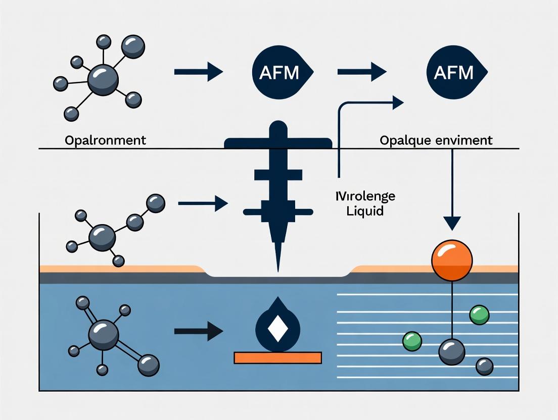
Q4: How does the signal generation and detection pathway differ between light microscopy and AFM for opaque samples? A: The fundamental pathways are completely distinct, as shown in the diagram below.
Light vs AFM Signal Pathways in Opaque Media
The Scientist's Toolkit: Research Reagent Solutions for Opaque Media AFM
| Item | Function / Rationale |
|---|---|
| Freshly Cleaved Mica Discs | Atomically flat, negatively charged substrate ideal for adsorbing biomolecules, cells, or hydrogels for stable AFM imaging. |
| Silicon Nitride AFM Probes (Soft Lever) | Probes with low spring constants (0.01-0.5 N/m) minimize sample damage, crucial for soft, biological samples in liquid. |
| Liquid Immersion Cell (Sealed) | Allows the probe and sample to be fully immersed in buffer or culture medium, maintaining biological viability during scanning. |
| Opaque Media-Compatible Buffer | A matched buffer or medium (e.g., PBS, cell culture media) to maintain sample integrity without interfering with probe mechanics. |
| Calibration Grating (e.g., TGZ1) | A standard sample with known pitch and height (e.g., 1 µm pitch, 20 nm depth) for verifying scanner accuracy and probe sharpness in Z-axis. |
| Vibration Isolation Table | Critical for high-resolution AFM; dampens environmental vibrations that cause noise, especially important for slow scans in liquid. |
This technical support center is framed within the thesis research on advancing Atomic Force Microscopy (AFM) for high-resolution imaging and force spectroscopy in opaque liquid environments, such as concentrated protein solutions, colloidal suspensions, and tissue cultures. The core principle leverages the AFM's mechanical probe (cantilever) to gather topographical and nanomechanical data without requiring optical transparency, overcoming a fundamental limitation of light-based microscopes.
Troubleshooting Guides & FAQs
Cantilever & Probe Issues
Q1: My cantilever response is erratic and noisy in an opaque biological fluid. What could be wrong? A: This is often caused by contamination or excessive hydrodynamic drag. Opaque media frequently have high viscosity and particulate content.
- Action 1: Check for Probe Contamination. Retract the probe and perform a cleaning protocol: Rinse in a series of solvents (e.g., ethanol, deionized water) appropriate for your sample. Use an ultrasonic cleaner for non-coated cantilevers cautiously (low power, <1 min).
- Action 2: Adjust Cantilever Choice. Switch to a higher resonance frequency cantilever in air to mitigate fluid damping effects. A stiffer cantilever (e.g., 1-10 N/m) may be necessary for penetrating viscous layers.
- Action 3: Optimize Imaging Parameters. Reduce the scan speed and increase the Integral Gain to maintain tracking. Engage at a lower setpoint.
Q2: How do I verify probe integrity and calibration in opaque liquid when I can't see it optically? A: Rely on the thermal tune and reference force curves.
- Protocol: In-Situ Thermal Tune Calibration.
- Fully submerge the probe in the liquid cell.
- Isolate the system from vibrations.
- Perform a thermal tune spectrum. The peak should be Lorentzian. A distorted peak suggests contamination or damage.
- Use the thermal tune to calibrate the spring constant (k) in the actual imaging fluid using the Sader or thermal noise method.
- Protocol: Reference Elasticity Measurement.
- Take force curves on a known, rigid substrate (e.g., cleaned glass or mica) immersed in the opaque liquid.
- The slope of the contact region should be linear and very steep. A reduced slope indicates a damaged or contaminated tip.
Sample & Imaging Issues
Q3: Sample drift is severe, preventing stable imaging in a temperature-controlled opaque liquid. A: Drift is exacerbated by thermal gradients and slow equilibration in dense liquids.
- Action 1: Extended Equilibration. After injecting the opaque liquid and sealing the cell, allow the system to equilibrate for at least 45-60 minutes before engaging.
- Action 2: Use a Liquid Cell with Active Temperature Stabilization. Ensure the heater/cooler is active well in advance.
- Action 3: Employ Drift Compensation Software. If available, use your AFM's linear or adaptive drift correction algorithms. Initial scans should be considered for drift measurement only.
Q4: How can I locate a specific region of interest on an opaque sample? A: You must use integrated stage microscopy or pre-marking.
- Protocol: Finder Grid Workflow.
- Pre-Marking: Use a finder grid (e.g., patterned substrate with coordinates) under an optical microscope to note the target location.
- Transfer: Mount the grid in the AFM liquid cell.
- Navigation: Use the AFM's coarse positioning stage to move to the approximate coordinates. Perform a large-area (e.g., 100x100 µm) low-resolution scout scan to identify the grid pattern and zero in on the target.
Data & Analysis Issues
Q5: Force curves collected in opaque media show an inconsistent baseline. How do I correct this? A: This is typically due to drift or a drifting laser photodiode alignment caused by refractive index changes.
- Action 1: Re-align the Laser. After liquid injection and equilibration, perform a fine laser alignment on the cantilever in the opaque liquid.
- Action 2: Post-Processing Correction. Use analysis software to subtract a linear or polynomial fit from the non-contact portion of each force curve.
- Action 3: Increase Approach/Velocity Rate. This minimizes the time for drift during the curve capture, but may not be suitable for all dynamic measurements.
Experimental Protocols Cited
Protocol 1: Imaging Lipid Bilayers in Concentrated Cell Lysate
- Objective: Visualize phase separation in supported lipid bilayers (SLBs) within an opaque, protein-rich environment.
- Method:
- Prepare SLBs on mica via vesicle fusion in a clear buffer.
- Inject concentrated cell lysate (opaque medium) into the fluid cell.
- Equilibrate for 60 minutes at 25°C.
- Engage in contact mode with a soft cantilever (0.1 N/m) at low force (setpoint ~0.5 nN).
- Scan at 1 Hz with a resolution of 512x512 pixels.
- Key Parameter Table:
Parameter Setting Rationale Cantilever Si₃N₄, 0.1 N/m Minimizes sample disturbance Mode Contact Mode Good for fluid, contiguous samples Scan Rate 1 Hz Compensates for fluid drag Setpoint 0.5 nN Low imaging force Temperature 25°C Stable, near-physiological
Protocol 2: Measuring Drug Particle Stiffness in Opaque Suspension
- Objective: Quantify nanomechanical changes in amorphous drug aggregates suspended in an opaque parenteral formulation.
- Method:
- Deposit 50 µL of the opaque formulation onto a polished steel substrate.
- Engage a stiff cantilever (40 N/m) in peak force tapping mode.
- Set peak force amplitude to 5-10 nN and frequency to 1 kHz.
- Map a 5x5 µm area, capturing topography and DMT modulus simultaneously.
- Use particle analysis software to extract modulus values for >100 individual particles.
- Key Parameter Table:
Parameter Setting Rationale Cantilever Diamond-coated, 40 N/m Penetrates viscous layer, robust Mode PeakForce QNM Quantitative nanomechanical mapping Peak Force 5-10 nN Sufficient for indentation Frequency 1 kHz Fast enough for stable mapping Analysis DMT Model Fits elastic modulus from retract curve
The Scientist's Toolkit: Research Reagent Solutions
| Item | Function in Opaque Liquid AFM |
|---|---|
| Silicon Nitride Probes (uncoated) | Standard for imaging soft biological samples; hydrophilic surface reduces non-specific binding. |
| Diamond-Coated Probes | Essential for stiff materials (e.g., bone, drug crystals) in abrasive media; extreme wear resistance. |
| Finder Grids (e.g., SPI Grids) | Patterned substrates with alphanumeric coordinates for relocating regions of interest without optics. |
| Temperature-Controlled Liquid Cell | Actively heats/cools sample to maintain physiological or process-relevant conditions, reducing drift. |
| Low-Autofluorescence Immersion Fluid | Used in combined AFM-confocal systems; minimizes background noise in the optical channel. |
| Inert, High-Density Fluid (e.g., Fluorocarbon) | Used as an immiscible overlay to seal the liquid cell, preventing evaporation of aqueous samples. |
| Biolayer Mimetics (e.g., SLB on Mica) | Provides a flat, biomimetic reference surface for calibration and control experiments in complex media. |
Visualizations
Diagram 1: AFM vs Optical Imaging in Opaque Media
Diagram 2: Opaque Liquid AFM Experiment Workflow
Diagram 3: Key Signals in AFM Opaque Imaging
Technical Support Center
FAQs & Troubleshooting for AFM Imaging in Opaque Liquid Environments
Q1: My AFM cantilever exhibits severe drift and instability when submerged in an opaque cell culture medium. What could be the cause and solution? A: This is often due to thermal drift from uneven heating or contamination of the cantilever/probe. Opaque media, like those containing phenol red or proteins, can absorb laser heat differently.
- Solution: Implement a thermal equilibration period of at least 45-60 minutes after fluid injection. Use tipless, silicon nitride cantilevers (e.g., Bruker MLCT-BIO-DC) with a reflective gold coating to enhance laser signal in low-visibility conditions. Perform a series of approach-retract cycles in a clear buffer first to check stability before introducing the opaque medium.
Q2: The laser deflection signal is lost upon engaging the sample in an opaque formulation. How can I regain detection? A: The primary cause is scattering or absorption of the laser beam by particulates or dense colorants in the liquid.
- Solution:
- Optimize the laser alignment at the liquid-air interface before adding the opaque solution.
- If possible, switch to a cantilever with a higher reflective coating or use a blue/violet laser (shorter wavelength) which may scatter less in some media.
- As a last resort, dilute the opaque formulation (e.g., 1:10 in PBS) to confirm functionality, though this may alter the sample's native state.
- Solution: Switch to PeakForce Tapping or QI Mode (Bruker) or AC Mode in liquid (Keysight, Asylum). These modes control the maximum applied force in the pN range. Start with a very low setpoint (e.g., 50-100 pN) and a soft cantilever (spring constant ~0.1 N/m). Use the following protocol for force calibration.
Q4: How do I verify my AFM calibration is accurate for force spectroscopy within a dense, opaque tissue matrix? A: Calibration in situ is critical. The hydrodynamic method is recommended for opaque liquids.
- Experimental Protocol: In-Liquid Cantilever Spring Constant Calibration via Thermal Tune Method:
- Setup: Engage the cantilever in the opaque liquid of interest, far from the sample surface (~10-20 µm).
- Data Acquisition: Record the thermal noise power spectrum over a 1 MHz bandwidth for 10 seconds.
- Analysis: Fit the fundamental resonance peak (typically 5-30 kHz in liquid) to a simple harmonic oscillator model. The area under the power spectral density curve is related to the mean square displacement via the Equipartition Theorem.
- Calculation: The spring constant k is calculated as k = kB T /
Q5: My bacterial biofilm samples in opaque nutrient broth move during scanning. How can I immobilize them without affecting viability? A: Physical entrapment is preferred over chemical fixation for live studies.
- Solution Protocol: Porous Membrane Immobilization:
- Use a track-etched polycarbonate membrane with 0.8 µm pores.
- Filter a dilute suspension of the biofilm cells/formulation onto the membrane under gentle vacuum.
- Carefully rinse with a compatible buffer to remove excess broth.
- Place the membrane, cell-side up, in the AFM liquid cell and submerge in the desired imaging liquid (e.g., fresh broth). The cells are physically trapped but remain hydrated and viable.
Data Presentation
Table 1: Performance of AFM Modes in Opaque Liquid Environments
| AFM Mode | Optimal Force Control Range | Best for Sample Type | Key Challenge in Opaque Liquids | Typical Resolution (XY) |
|---|---|---|---|---|
| Contact Mode | 0.5 - 10 nN | Rigid polymers, crystals | High shear forces cause sample deformation/drag | 5-10 nm |
| Tapping Mode (in liquid) | 0.1 - 1 nN | Adsorbed proteins, fixed cells | Maintaining oscillation; laser instability | 2-5 nm |
| PeakForce Tapping | 10 - 500 pN | Live cells, hydrogels, vesicles | Finding initial setpoint without visual aid | 1-3 nm |
| Force Spectroscopy | 10 - 10,000 pN | Molecular bonds, local elasticity | Drift during long approach-retract cycles | N/A (point measurement) |
Table 2: Recommended Cantilevers for Opaque Liquid Imaging
| Cantilever Model (Maker) | Material | Spring Constant (N/m) | Resonant Freq. in Liquid (kHz) | Key Feature for Opaque Media |
|---|---|---|---|---|
| MLCT-BIO-DC (Bruker) | SiN | 0.03 - 0.06 | ~8-12 | Reflective gold back-side coating |
| Biolever Mini (Olympus) | SiN | 0.03 - 0.06 | ~15-25 | High reflection, sharp tip |
| qp-BioAC (Nanosensors) | Si | 0.07 - 0.3 | ~20-40 | Very sharp tip for high-res |
| TR400PSA (Asylum) | SiN | 0.02 - 0.08 | ~9-14 | Long, reflective tip for deep cells |
Experimental Protocols
Protocol: Mapping Drug Release from a Nanoparticle in Simulated Opaque Biological Fluid Objective: To spatially map the change in mechanical properties of a polymeric nanoparticle during drug release in an opaque medium (e.g., simulated intestinal fluid with bile salts).
- Sample Preparation: Deposit Poly(lactic-co-glycolic acid) (PLGA) nanoparticles on a freshly cleaved mica substrate. Treat with 0.1% poly-L-lysine for 5 minutes to enhance adhesion.
- AFM Setup: Mount the sample in the fluid cell. Inject clear PBS buffer. Engage using a soft cantilever (k ~0.1 N/m) in PeakForce Tapping mode. Locate and image a single nanoparticle.
- Baseline Measurement: Acquire a high-resolution force map (256x256 pixels) over a 500x500 nm area on the nanoparticle. Record the DMT modulus for each pixel.
- Introduce Opaque Medium: Gently retract the tip. Flush the liquid cell with 3x its volume with pre-warmed (37°C), opaque simulated intestinal fluid (FaSSIF).
- Time-Lapse Imaging: Re-engage near the same nanoparticle. Acquire successive force maps at 5, 15, 30, and 60-minute intervals using identical imaging parameters.
- Data Analysis: Use offline software to calculate the average Young's modulus of the nanoparticle at each time point. Plot modulus vs. time to infer drug release kinetics based on polymer softening.
The Scientist's Toolkit: Research Reagent Solutions
| Item | Function in AFM of Opaque Liquids |
|---|---|
| Silicon Nitride Cantilevers (tipless, reflective) | Minimize fluid drag; enhance laser reflectivity for stable detection in scattering media. |
| Track-Etched Polycarbonate Membranes (0.4-1.0 µm pores) | Immobilize live cells, tissues, or particles without chemical fixation for in-situ liquid imaging. |
| Poly-L-Lysine Solution (0.01%-0.1%) | Treats substrates (mica, glass) to promote electrostatic adhesion of negatively charged samples (cells, nanoparticles). |
| Simulated Biological Fluids (FaSSIF/FeSSIF) | Opaque, biorelevant media for studying drug formulations in physiologically accurate environments. |
| Temperature Control Stage (Petri Dish Heater) | Maintains sample viability and reduces thermal drift, a major source of instability in liquid. |
| Blue/Violet Laser Diode Module (Upgrade) | Shorter wavelength scatters less than standard red laser in some turbid media, improving signal-to-noise. |
Visualizations
Title: Workflow for AFM Experiments in Opaque Liquids
Title: Key Challenges in AFM of Opaque Media
This technical support center is framed within a thesis on advancing Atomic Force Microscopy (AFM) imaging in opaque liquid environments. Opaque liquids, such as emulsions, suspensions, and complex biological fluids (e.g., blood, synovial fluid, cell lysates), present significant challenges for high-resolution imaging due to light scattering and probe instability. This guide provides troubleshooting and methodologies for researchers navigating these challenges.
Troubleshooting Guide & FAQs
Q1: My AFM cantilever shows erratic deflection and high noise in a dense bacterial suspension. What could be the cause? A: This is likely due to non-specific adhesion of particles or cells to the cantilever and tip. The suspended microorganisms cause intermittent probe collisions and damping.
- Solution: Implement a two-step protocol: (1) Use a tipless cantilever to first map the general topography and fluid density via force spectroscopy. (2) Switch to a sharp, hydrophobic-coated tip (e.g., Si-N with octadecyltrichlorosilane) for detailed imaging, reducing adhesion. Reduce scan speed to <0.5 Hz.
Q2: How can I verify if my emulsion sample is stable enough for AFM imaging without phase separation during a scan? A: Perform a pre-imaging stability assay using dynamic light scattering (DLS).
- Solution: Measure the droplet size distribution via DLS at 25°C every 15 minutes for 2 hours. A stable emulsion for AFM will have a polydispersity index (PDI) below 0.2 and a change in Z-average diameter of <5% over time. If instability is detected, increase surfactant concentration by 0.1% w/v and re-homogenize.
Q3: I am getting no contrast when imaging protein aggregates in an opaque synovial fluid simulant. What should I adjust? A: The issue is likely insufficient mechanical contrast between the soft aggregates and the viscous fluid medium.
- Solution: Employ PeakForce Tapping mode with a stiff cantilever (k ~ 40-80 N/m). Adjust the peak force setpoint to the lower 10-15% of the force-distance curve slope to ensure consistent tip-sample interaction. Use a modulation frequency of 2 kHz to penetrate the fluid layer.
Q4: What is the best method to immobilize lipid nanoparticles in an opaque suspension for AFM without drying artifacts? A: Use a functionalized substrate that promotes weak electrostatic immobilization.
- Solution: Prepare a poly-L-lysine coated mica substrate. Dilute the nanoparticle suspension 1:10 in a low-conductivity buffer (1 mM HEPES, pH 7.4). Incubate 10 µL on the substrate for 5 minutes, then gently introduce into the fluid cell with excess imaging buffer to remove loosely bound particles.
Q5: My probe frequently crashes when approaching the surface in whole blood samples. How can I prevent this? A: The approach is hindered by a dense matrix of red blood cells and proteins.
- Solution: Use a "blind" approach mode with a very low setpoint (<< 0.5 V). Alternatively, pre-treat the sample by centrifugation at 500 g for 5 minutes to create a cell-free plasma layer near the substrate surface. Image within this top layer. Consider using a colloidal probe tip (sphere radius ~5µm) for greater robustness.
Table 1: Common Opaque Liquids & AFM Imaging Parameters
| Liquid Type | Example | Typical Viscosity (cP) | Recommended AFM Mode | Optimal Cantilever Stiffness | Max Practical Scan Size |
|---|---|---|---|---|---|
| Oil-in-Water Emulsion | Paraffin/Water, 10% | ~3-5 | PeakForce Tapping / QNM | 0.7 - 2 N/m | 10 x 10 µm |
| Pharmaceutical Suspension | Drug nanocrystals (10 mg/mL) | ~8-15 | Contact Mode (Fluid) | 0.1 - 0.4 N/m | 5 x 5 µm |
| Biological Fluid | Undiluted Synovial Fluid | ~500-10000 | PeakForce Tapping | 20 - 80 N/m | 2 x 2 µm |
| Cell Culture Lysate | HEK293 Lysate | ~10-30 | Fast Force Mapping | 0.4 - 1 N/m | 20 x 20 µm |
| Whole Blood (Diluted 1:10) | Human Blood in PBS | ~1.5-2 | Non-Contact / AC Mode | 7 - 20 N/m | 15 x 15 µm |
Table 2: Troubleshooting Matrix: Symptom vs. Solution
| Symptom | Likely Cause | Immediate Action | Long-term Protocol Adjustment |
|---|---|---|---|
| High thermal drift (>50 nm/min) | Temperature gradient in fluid | Allow 30 min thermal equilibration in chamber | Use a temperature controller stage (±0.1°C) |
| Image appears "smeared" | Probe dragging/fluid drag | Increase retract velocity by 50% | Switch to a higher resonance frequency cantilever |
| Sudden loss of signal | Contaminated probe or substrate | Retract, clean fluid cell with 2% Hellmanex | Implement inline syringe filtration (0.2 µm) of imaging buffer |
| Inconsistent modulus readings | Heterogeneous liquid density | Increase peak force frequency to sample faster | Perform 100-point force curve grid prior to imaging for mapping |
Experimental Protocols
Protocol 1: Immobilizing and Imaging Liposomes in an Opaque Serum Medium
- Substrate Preparation: Cleave a mica disk. Apply 50 µL of 0.1% w/v polyethyleneimine (PEI) solution for 1 minute. Rinse with DI water and dry under nitrogen.
- Sample Preparation: Dilute the liposome-serium mixture 1:5 in isotonic sucrose solution (300 mOsm). Gently agitate.
- Immobilization: Pipette 20 µL of diluted sample onto the PEI-coated mica. Incubate in a humidity chamber for 15 minutes.
- AFM Mounting: Do not rinse. Carefully mount the substrate into the fluid cell, avoiding air bubbles. Add 1 mL of the 1:5 dilution serum-sucrose solution as imaging buffer.
- Imaging: Engage in PeakForce Tapping mode with a cantilever (k=0.6 N/m, f0~65 kHz in fluid). Set peak force amplitude to 5-10 nN. Scan at 0.8 Hz.
Protocol 2: Characterizing Aggregate Size in a Turbid Formulation
- Calibration: Image a grating (e.g., TGZ1) in the same opaque liquid to calibrate the scanner's x, y, and z axes for fluid damping effects.
- Imaging: Deposit 30 µL of the undiluted turbid formulation on clean glass. Use a sharp tip (k=40 N/m) in Fast Force Mapping mode.
- Data Acquisition: Perform a 50 x 50 µm scan with 256x256 pixels, acquiring a force-distance curve at each point.
- Analysis: Use the software's particle analysis toolkit. Set a modulus threshold (e.g., >1 GPa for hard aggregates) to differentiate aggregates from the softer formulation matrix. Export aggregate diameter and circularity data.
Visualizations
Title: AFM Workflow for Opaque Liquid Samples
Title: Opaque Fluid Effect on AFM Signal Pathway
The Scientist's Toolkit: Research Reagent Solutions
Table 3: Essential Materials for AFM in Opaque Liquids
| Item | Function/Benefit | Example Product/Brand |
|---|---|---|
| Functionalized Mica Disks | Provides a flat, charged surface for immobilizing particles, vesicles, or biomolecules from suspension. | PEI-Coated Mica, PLL-Coated Mica (Novascan) |
| Hydrophobic Cantilever Coatings | Minimizes non-specific adhesion of biomolecules in complex fluids like serum or lysate. | OTS-coated Si3N4 tips |
| High-Stiffness Cantilevers (k > 40 N/m) | Necessary for penetrating viscous layers and for PeakForce Tapping in stiff gels. | Bruker RTESPA-150, Olympus AC240TS |
| Syringe Fluid Filters (0.1/0.2 µm) | Filters imaging buffer in-line to remove particulates that could contaminate the tip or sample. | Whatman Anotop 10 (0.1 µm Pore) |
| Temperature Control Stage | Stabilizes thermal drift in non-homogeneous, viscous liquids during long scans. | Bruker BioHeater, JPK PetriScan Heater |
| Low-Adhesion Colloidal Probes | Spherical tips for robust imaging in dense suspensions and accurate rheology measurements. | 5µm Silica Sphere Probes (Novascan) |
| Isotonic Sucrose/HEPES Buffer | Provides imaging medium that minimizes osmotic stress to biological specimens without adding ions that interfere with AFM. | 300 mOsm Sucrose, 1 mM HEPES, pH 7.4 |
Troubleshooting Guides & FAQs
Cantilever & Tip Issues
Q1: Why am I getting excessively high deflection noise or 'jumpy' data when imaging in liquid? A: This is often due to cantilever resonance excitation from fluid motion or improper acoustic isolation. First, ensure the liquid cell is firmly sealed and all air bubbles are purged. Allow the system to thermally equilibrate for at least 30-60 minutes. Use cantilevers with lower spring constants (e.g., 0.1 - 0.5 N/m) to reduce sensitivity to turbulence. Employing a higher drive frequency (if in tapping mode) away from major mechanical resonances of the fluid cell can also help.
Q2: My tip appears blunt or contaminated quickly during liquid imaging. How can I mitigate this? A: Tip degradation in liquid is accelerated by adhesive samples and contaminants. Use sharper, non-coated silicon nitride (SiN) tips for soft biological samples. Implement a brief in-situ cleaning protocol: after loading, oscillate the tip at high amplitude in clean buffer for 2-3 minutes before engaging. For persistent contamination, a mild piranha etch (only for silicon tips) is a last resort but requires complete re-calibration.
Q3: What causes inconsistent tapping mode phase contrast or failure to maintain oscillation in liquid? A: This typically stems from incorrect drive frequency selection or damping. Always perform a thermal tune in the specific liquid to find the true resonance peak, as it shifts significantly from air. Reduce the drive amplitude to minimize tip-sample forces that can quench oscillation. If the problem persists, increase the setpoint (reduce engagement force) and verify that your cantilever's Q-factor is suitable for liquid (low Q, ~1-5).
Liquid Cell & Environment Issues
Q4: How do I eliminate drift and instability during long-term imaging in an opaque liquid? A: Drift in opaque liquids (like cell culture media) is exacerbated by thermal gradients and concentration changes. Use a temperature-controlled stage (±0.1°C stability). Ensure the liquid is fully degassed to prevent bubble formation. A key protocol is to incubate the entire fluid cell assembly at the experiment temperature for one hour prior to sample injection. Employ closed-loop scanner systems when possible.
Q5: My sample detaches from the substrate during liquid exchange or scanning. How can I improve sample adhesion? A: Substrate functionalization is critical. For proteins or cells, use coated substrates (e.g., poly-L-lysine, APTES for silanes). A detailed protocol: Clean a glass coverslip with oxygen plasma for 5 minutes. Incubate with 0.1% poly-L-lysine solution for 30 minutes. Rinse gently with DI water and dry with inert gas. Let substrate sit in imaging buffer for 15 minutes before sample deposition to stabilize the surface.
Q6: Air bubbles are trapped under the cantilever chip, causing erratic behavior. What is the proper priming procedure? A: Follow this step-by-step priming protocol: 1) With the cantilever holder outside the scanner, inject buffer via the inlet port until a large drop forms at the outlet. 2) Tilt the holder to ~45 degrees and gently insert the cantilever chip into the drop, allowing capillary action to wet the chip back. 3) Secure the holder in the scanner. 4) Use syringe pumps to slowly exchange fluid at 50 µL/min for at least 3 volume exchanges of the cell.
Table 1: Cantilever Selection Guide for Liquid Imaging
| Material | Typical Spring Constant (N/m) | Resonance Freq in Liquid (kHz) | Best For | Key Limitation |
|---|---|---|---|---|
| Silicon Nitride (SiN) | 0.06 - 0.6 | 5 - 40 | Bio-molecules, live cells (Contact/Tapping) | Lower stiffness limits use on stiff materials |
| Silicon (Si) | 1 - 40 | 20 - 150 | Polymers, electrochemistry (Tapping/PeakForce) | More hydrophobic, can have higher adhesion |
| Quartz (qPlus) | 1,000 - 10,000 | N/A (FM-AFM) | Atomic resolution in liquid | Complex setup, very specialized |
Table 2: Liquid Cell Modalities & Performance Parameters
| Cell Type | Volume (µL) | Flow Control | Max Scan Size | Suitability for Opaque Liquids |
|---|---|---|---|---|
| Open Dish | 500 - 2000 | Poor (passive) | ~100 µm | Poor (evaporation, contamination) |
| Sealed Cell (O-ring) | 30 - 100 | Good (ports) | ~50 µm | Good (if chemically compatible) |
| Microfluidic Cell | 1 - 10 | Excellent (pumps) | ~20 µm | Excellent (rapid exchange, temp control) |
Experimental Protocols
Protocol 1: In-Liquid Cantilever Tuning for Opaque Media
- Mount and Prime: Install the cantilever and liquid cell, prime thoroughly to remove bubbles.
- Thermal Tune: With the tip disengaged, command a thermal spectrum acquisition. Set frequency range to 5-400 kHz.
- Peak Identification: Fit the resonance peak to a simple harmonic oscillator model. Record the peak frequency (f_res) and quality factor (Q).
- Drive Setting: Set the drive frequency to f_res. Set drive amplitude to 50-100 mV initially.
- Engagement: Engage using a setpoint of ~0.8-0.9 of the free amplitude (for tapping mode).
Protocol 2: Sample Preparation for Lipid Bilayer Imaging in Buffer
- Substrate Cleaning: Sonicate mica discs in isopropanol, then DI water, for 5 minutes each. Dry with N2.
- Bilayer Deposition: Use a vesicle fusion method. Inject 100 µL of 0.1 mg/mL small unilamellar vesicle (SUV) solution onto freshly cleaved mica.
- Incubation: Incubate for 30 minutes at 60°C in a humid chamber.
- Rinsing: Rinse the mica surface with 2 mL of imaging buffer (e.g., 150 mM NaCl, 10 mM HEPES, pH 7.4) to remove unfused vesicles.
- Loading: Immediately mount the mica in the AFM liquid cell, fill with imaging buffer, and proceed to imaging.
Visualizations
Diagram 1: Liquid AFM Setup Workflow
Title: Liquid AFM Experiment Setup Sequence
Diagram 2: Key Forces in Liquid AFM Imaging
Title: Force Interactions During Liquid AFM Scanning
The Scientist's Toolkit: Research Reagent Solutions
| Item | Function in Liquid AFM Experiment |
|---|---|
| SiN Cantilevers (e.g., MLCT-BIO) | Low spring constant minimizes sample damage. Hydrophilic surface reduces non-specific adhesion in buffer. |
| Poly-L-Lysine Solution (0.1%) | Coats negatively charged substrates (glass/mica) to promote adhesion of cells or tissue samples. |
| HEPES Buffered Saline (20 mM, pH 7.4) | Maintains physiological pH without CO2 control, crucial for live-cell imaging in opaque media. |
| Bovine Serum Albumin (BSA, 1%) | Used as a blocking agent to passivate substrates and fluid cell components, reducing sample contamination. |
| Degassed DI Water / Buffer | Prevents nucleation and growth of air bubbles under the cantilever during scanning, a major source of noise. |
| Oxygen Plasma Cleaner | Creates a pristine, hydrophilic surface on substrates and cantilever chips prior to functionalization. |
| Syringe Pump System | Enables precise, low-flow-rate fluid exchange within sealed cells for drug addition or buffer changes. |
| Temperature Controller | Stabilizes the sample environment, minimizing thermal drift during long experiments in incubating media. |
Practical Guide: Modes, Setups, and Real-World Applications in Drug and Bio Research
This technical support center is framed within a broader thesis on advancing Atomic Force Microscopy (AFM) for high-resolution imaging in opaque liquid environments, critical for research in biophysics and drug development. Selecting between Contact and Tapping Mode is a fundamental decision that dictates data quality and sample integrity.
Troubleshooting Guides & FAQs
Q1: My image in liquid Contact Mode shows severe streaks and sample dragging. What is the cause and solution? A: This is typically caused by excessive lateral forces and high adhesion between the tip and sample.
- Troubleshooting Steps:
- Reduce Applied Force: Immediately lower the setpoint force. Engage at a higher setpoint and gradually decrease it until the tip maintains contact with minimal deflection.
- Check Cantilever Spring Constant: Use a softer cantilever (k < 0.1 N/m) to minimize applied force.
- Modify Liquid Environment: Add ions (e.g., 25-150 mM NaCl) to your buffer to screen electrostatic interactions, or consider a surfactant (e.g., 0.1% pluronic) to reduce hydrophobic adhesion.
- Switch to Tapping Mode: If dragging persists, the sample may be too soft; Tapping Mode is the recommended alternative.
Q2: In liquid Tapping Mode, my cantilever oscillation amplitude is unstable and decays over time. How do I fix this? A: Amplitude decay often indicates fluid damping or contamination.
- Troubleshooting Steps:
- Clean the Cantilever: Perform UV-ozone cleaning for 15-20 minutes before use, or use plasma cleaning.
- Adjust Drive Frequency: Manually find the peak in the amplitude-frequency curve in liquid, as it shifts significantly from the air resonance.
- Optimize Drive Amplitude: Increase the drive amplitude to compensate for heavy damping in viscous liquids.
- Reduce Scan Speed: Lower the scan speed to allow the feedback loop to track the surface correctly.
- Check for Bubbles: Ensure no air bubbles are trapped on the cantilever chip or fluid cell; degas buffers before use.
Q3: When imaging live cells in opaque media, which mode provides better viability and resolution? A: Tapping Mode is overwhelmingly preferred for live cells.
- Reasoning: It eliminates the destructive lateral shear forces of Contact Mode. The intermittent contact minimizes sample disturbance, maintaining cell viability for longer-term experiments. Use low amplitudes (A0 < 10 nm) and setpoints >80% of A0 for gentle imaging.
Quantitative Comparison Table
| Parameter | Contact Mode in Liquid | Tapping Mode in Liquid |
|---|---|---|
| Lateral Force | High (can cause dragging) | Very Low |
| Normal Force Control | Direct via deflection setpoint | Indirect via amplitude setpoint |
| Typical Resolution | High on rigid samples | High on soft & rigid samples |
| Sample Damage Risk | High for soft samples (e.g., cells, membranes) | Low |
| Recommended Cantilever k | Very Soft (0.01 - 0.1 N/m) | Soft to Medium (0.1 - 1 N/m) |
| Optimal Drive Frequency | Not Applicable (DC mode) | ~10-15% below in-air resonance |
| Best For | Atomic-resolution on hard materials (mica, HOPG), force spectroscopy | Soft samples (proteins, live cells, polymers), rough surfaces |
Experimental Protocols
Protocol 1: Calibrating Cantilevers for Quantitative Liquid-Phase Imaging
- Thermal Tune Method: Acquire the thermal power spectrum of the cantilever in the target liquid.
- Fit the Data: Fit the fundamental resonance peak to a simple harmonic oscillator model to obtain the resonance frequency (f_res) and quality factor (Q).
- Calculate Spring Constant: Use the Sader method or the thermal noise method, inputting f_res, Q, and the fluid's viscosity/density.
- Sensitivity Measurement: Ramp the tip against a rigid substrate (e.g., sapphire) in liquid to obtain the deflection sensitivity (nm/V).
Protocol 2: Imaging Membrane Proteins in Opaque Buffer
- Sample Preparation: Deposit proteoliposomes or supported lipid bilayers containing the protein of interest onto freshly cleaved mica.
- Fluid Cell Assembly: Use a sealed liquid cell to prevent evaporation. Inject >1 mL of opaque buffer (e.g., containing suspended carriers) to fully exchange the medium.
- Mode Selection: For protein topography, use Tapping Mode. Engage with low amplitude (~1-2 V, ~5 nm). Set drive frequency to the liquid resonance peak.
- Imaging Parameters: Set scan size to 1-2 µm, scan rate to 1-2 Hz, and amplitude setpoint to 85-90% of the free amplitude.
- Data Acquisition: Capture 512x512 pixel images. Use a line-by-line leveling filter during acquisition.
Visualization: AFM Mode Selection Logic for Liquid Imaging
Title: Decision Logic for AFM Mode Selection in Liquid
The Scientist's Toolkit: Research Reagent Solutions
| Item | Function & Rationale |
|---|---|
| Soft Silicon Nitride Cantilevers (k ~0.06 N/m) | Low spring constant minimizes indentation force on soft samples in Contact Mode and enables stable oscillation in Tapping Mode. |
| NP-S or DNP-S Probes | Sharp, silicon nitride tips optimized for imaging in fluids with standard shapes for consistent performance. |
| Pluronic F-127 Surfactant | Added at 0.1% w/v to buffers to passivate tips and substrates, reducing non-specific adhesion and sample drag. |
| Degassed Imaging Buffer | Prevents nucleation of air bubbles on the cantilever during data acquisition, which destabilizes oscillation. |
| UV-Ozone Cleaner | Critical for removing organic contaminants from cantilever chips before use, ensuring predictable wetting and oscillation. |
| Sealed Liquid Cell with O-Rings | Allows for complete containment of opaque or volatile liquids and prevents evaporation during long scans. |
| Calibration Gratings (e.g., TGZ1, XGRW) | Used for in-situ verification of scanner accuracy and image dimensions in the Z-axis within the liquid cell. |
Technical Support Center
Troubleshooting Guide & FAQs
Q1: The AFM cantilever becomes contaminated or gives inconsistent readings immediately after immersion in my opaque drug solution. What could be the issue?
A: This is often caused by poor sample preparation or an unsuitable immersion protocol. Opaque solutions, such as concentrated protein suspensions or lipid-based drug carriers, frequently contain aggregates or surfactants that rapidly adsorb onto the probe and sample surface. First, ensure the solution is centrifuged (see Protocol 1) to remove large particulates. Second, modify the immersion sequence: approach the probe to the sample surface in a clean buffer first, then gently exchange the liquid to the opaque solution using a micro-syringe pump to minimize convective adsorption. Always perform an in-situ cleaning procedure (tapping in clean buffer for 10 minutes) on a dummy area before engaging on your target scan area.
Q2: How do I verify the integrity of my substrate and adsorbed sample layer before imaging in an opaque liquid? I cannot use optical microscopy.
A: Implement a pre-scan verification protocol using AFM itself. Before introducing the opaque solution, image your substrate (e.g., mica, functionalized glass) in air or a clear buffer in Contact or Tapping Mode to confirm cleanliness and flatness. Then, adsorb your sample (e.g., vesicles, particles) from the opaque solution and rinse with a compatible clear buffer to remove bulk opacity. Perform a second scan in the clear buffer to confirm sample adhesion and distribution. Finally, carefully re-introduce the opaque solution for your experimental scans. This multi-step verification is critical for distinguishing sample features from debris.
Q3: My opaque solution (e.g., a melanin suspension) causes excessive laser drift on my AFM. How can I stabilize the system?
A: Opaque, light-absorbing solutions cause localized heating and thermal drift. Key mitigation steps include:
- Thermal Equilibration: Allow the fluid cell and solution to sit on the scanner for a minimum of 45 minutes before engagement.
- Use a Shrouded Cantilever: Choose a probe with a reflective coating on the backside only, minimizing a "sail" effect from convective currents.
- Reduce Laser Power: Lower the photodetector's laser power to the minimum acceptable level to reduce heating.
- Protocol Adjustment: Employ slower engage and scan speeds (e.g., 0.5 Hz) for the first few scans to allow stabilization. Data on thermal stabilization times under different conditions are summarized in Table 1.
Table 1: Thermal Drift Stabilization Times in Opaque Solutions
| Solution Type | Typical Concentration | Recommended Equilibration Time (mins) | Reduction in Drift Rate (nm/min) |
|---|---|---|---|
| Lipid Vesicles (MLV) | 5 mg/mL | 45 | 15.2 → 2.1 |
| Carbon Black Dispersion | 1% w/w | 60+ | 28.7 → 3.5 |
| Protein Aggregates | 10 mg/mL | 30 | 8.5 → 1.3 |
| Polymer Microgel | 2% w/w | 40 | 12.4 → 2.8 |
Experimental Protocols
Protocol 1: Sample Clarification for Opaque Solutions
- Purpose: Remove large aggregates that cause tip contamination.
- Materials: Opaque sample solution, micro-centrifuge, centrifuge filters (100 kDa or 0.22 µm pore, depending on sample).
- Method: 1) Load 500 µL of solution into a centrifugal filter unit. 2) Centrifuge at 5000 x g for 10 minutes at the solution's storage temperature. 3) Carefully extract the filtrate (for removing aggregates) or the retentate (for collecting clarified concentrate) using a pipette. Avoid disturbing the pelleted material. 4) Proceed to substrate preparation.
Protocol 2: Sequential Immersion for Stable Imaging
- Purpose: Achieve stable probe immersion and minimize surface contamination.
- Materials: AFM with liquid cell, syringe pump with tubing, clean buffer, clarified opaque solution.
- Method: 1) Mount the sample and probe in the liquid cell. 2) Inject 1 mL of clean buffer to fill the cell. 3) Engage the probe onto the surface in tapping mode and allow thermal stabilization for 20 mins. 4) Start a slow scan (1 Hz) on a 1 µm² area. 5) Using a syringe pump at 50 µL/min, perfuse 2 mL of the opaque solution through the cell. 6) Continue scanning, allowing 15 minutes for a new thermal equilibrium. 7) Move to the desired scan area.
The Scientist's Toolkit: Research Reagent Solutions
| Item | Function in Opaque Solution AFM |
|---|---|
| Functionalized Mica Discs | Provides an atomically flat, positively or negatively charged substrate to immobilize particles/vesicles from opaque solutions for imaging. |
| Syringe Pump & Micro-Tubing | Enables precise, low-flow-rate exchange of opaque solutions in the AFM liquid cell, minimizing shear forces that could displace samples. |
| Centrifugal Filter Units | Key for clarifying stock solutions by removing large aggregates that are common in opaque formulations and are primary sources of tip contamination. |
| Low-Adsorption Pipette Tips | Reduces loss of expensive or scarce sample material (e.g., drug delivery liposomes) onto plastic surfaces during handling. |
| Cantilevers with High Coating Reflectivity | Maximizes laser signal in sub-optimal conditions caused by light-scattering from the opaque medium, improving detection stability. |
Workflow Diagrams
Title: AFM Imaging Workflow for Opaque Liquid Samples
Title: Troubleshooting Logic for Opaque Solution AFM Issues
Technical Support Center: AFM Imaging in Liquid Environments
Troubleshooting Guides
Issue 1: Unstable or Drifting Probe During Imaging in Opaque Liquid Problem: The AFM cantilever shows excessive drift or instability, preventing clear imaging of liposomes in cell culture media or other opaque buffers. Diagnosis & Solution:
| Potential Cause | Diagnostic Check | Recommended Action |
|---|---|---|
| Thermal or Mechanical Drift | Monitor baseline deflection in contact mode over 5 minutes without sample. | Allow system to thermally equilibrate for 60+ minutes. Use a vibration isolation table. Enclose the AFM head with a acoustic hood. |
| Insufficient Probe Immersion | Visually check if the liquid fully covers the cantilever and its base. | Ensure liquid droplet is sufficiently large (typically 50-100 µL). Use a liquid cell or O-ring to contain the fluid if available. |
| High Ionic Strength/Liquid Opacity | Check for excessive laser deflection noise or low sum signal. | Dilute the opaque liquid if possible (e.g., 1:2 with buffer). Use a cantilever with a higher reflective coating. Switch to a specialized liquid probe (e.g., PNPLA). |
| Sample Adhesion Failure | Observe if particles are swept away by the probe. | Use a freshly cleaved mica surface functionalized with 0.1% poly-L-lysine for 5 minutes to improve carrier adhesion before washing. |
Issue 2: Low Resolution or "Smearing" of Nanoparticles Problem: Acquired images of polymeric micelles or SLNs appear blurred, lack distinct boundaries, or show smearing artifacts. Diagnosis & Solution:
| Potential Cause | Diagnostic Check | Recommended Action |
|---|---|---|
| Excessive Imaging Force | Check setpoint ratio. In contact mode, monitor deflection error. | Reduce the setpoint to apply minimal force (often < 0.5 nN). Use Tapping Mode in liquid (AC mode) to eliminate lateral shear forces. |
| Inappropriate Scan Speed | Image shows streaking in the fast-scan direction. | Decrease scan speed. For 1 µm scans, use 0.5-1.0 Hz. For high-resolution imaging of 100 nm carriers, use 2-4 Hz. |
| Probe Contamination | Perform a frequency sweep in liquid; resonant peak is broadened or shifted. | Clean the probe and sample stage with solvents (ethanol, isopropanol). Use UV-ozone cleaning for the probe holder. Replace the cantilever. |
| Carrier Softness/Deformation | Height measurements are inconsistent and lower than expected from DLS. | Operate in PeakForce Tapping or QI mode to minimize deformation. Use the softest available cantilevers (spring constant ~0.1 N/m). |
Issue 3: Inability to Locate or Identify Carriers on the Substrate Problem: The substrate appears featureless despite the confirmed presence of nano-carriers in the dispersion. Diagnosis & Solution:
| Potential Cause | Diagnostic Check | Recommended Action |
|---|---|---|
| Low Particle Density | Perform a wide-area scan (e.g., 20x20 µm). | Increase sample concentration. Incubate a 10-20 µL droplet of the nano-carrier solution on the substrate for 15-30 minutes, then gently rinse with DI water to remove unbound carriers. |
| Substrate Roughness | Image the substrate alone; RMS roughness exceeds 1 nm. | Use atomically flat substrates: freshly cleaved mica, highly ordered pyrolytic graphite (HOPG), or template-stripped gold. |
| Carrier Transparency in Fluid | Difficulty maintaining feedback on features. | Adjust the feedback gains (increase integral gain slightly). Use phase imaging in Tapping Mode to enhance material contrast. |
| Aggregation Clustering | Features are large and irregular. | Filter the nano-carrier dispersion through a 0.22 µm or 0.45 µm syringe filter (compatible with lipid/polymer) immediately before deposition. |
Frequently Asked Questions (FAQs)
Q1: What is the optimal AFM mode for imaging soft nano-carriers like liposomes in opaque biological fluids? A: For high-resolution imaging in opaque liquids, PeakForce Tapping (Bruker) or Quantitative Imaging (QI) Mode (Keysight) is generally optimal. These modes provide direct control over the maximum applied force (<100 pN possible), minimizing sample deformation. If these are unavailable, AC Mode (Tapping Mode) in liquid with a very low amplitude setpoint (70-80% of free amplitude) is the next best option. Contact mode is not recommended for soft carriers due to high lateral forces.
Q2: How do I prepare mica for adsorbing cationic liposomes? A: Protocol: 1) Cleave Mica: Use adhesive tape to expose a fresh, atomically flat surface. 2) Deposit Sample: Apply 20 µL of liposome suspension (diluted to ~0.1 mg/mL lipid in a low-salt buffer like 10 mM HEPES) onto the mica. 3) Incubate: Allow adsorption for 10-15 minutes in a humid chamber to prevent evaporation. 4) Rinse: Gently rinse the surface with 2-3 mL of ultrapure water or imaging buffer to remove unadsorbed liposomes and salts. 5) Blot: Carefully blot the edges with a lint-free tissue to leave a thin liquid film. 6) Mount: Immediately transfer to the AFM liquid cell and proceed with imaging.
Q3: My measured SLN height from AFM is significantly less than the hydrodynamic diameter from DLS. Why? A: This is a common artifact due to tip convolution and sample deformation. Quantitative data from recent studies (2023-2024) is summarized below:
| Nano-Carrier Type | Reported DLS Size (nm) | Reported AFM Height (nm) | Typical Deformation/Compression | Primary Cause |
|---|---|---|---|---|
| Solid Lipid Nanoparticle (SLN) | 120 ± 15 | 85 ± 10 | ~30% | High imaging force, tip pressing into soft lipid matrix. |
| Polymeric Micelle (PEG-PLGA) | 65 ± 5 | 55 ± 4 | ~15% | Moderate deformation of polymer core. |
| Liposome (DPPC) | 90 ± 10 | 88 ± 9 | ~2% | Fluid bilayer less prone to compression under low force. |
Solution: Use the lowest possible imaging force and measure particle height, not width. Width is overestimated due to tip geometry.
Q4: Can I image nano-carriers directly in whole blood or serum using AFM? A: Direct imaging in whole blood is extremely challenging due to high opacity, viscosity, and non-specific adhesion of blood components. A validated protocol involves: 1) Sample Preparation: Dilute serum 1:10 or 1:20 with PBS. 2) Substrate Functionalization: Use a chemically modified substrate (e.g., mica functionalized with a specific antibody or polyethylene glycol (PEG) to selectively capture carriers and resist protein fouling). 3) Imaging Mode: Use high-speed AFM or fast-scanning modes to overcome some drift. However, most research for opaque environments uses model opaque media (e.g, 1% BSA in PBS, concentrated protein solutions) rather than whole blood.
Q5: Which cantilevers are best for high-resolution imaging of micelles in liquid? A: See "The Scientist's Toolkit" below for specific recommendations. The key parameters are: Low spring constant (0.1 - 0.7 N/m) to minimize deformation, high resonant frequency in liquid (>10 kHz) for stability, and a sharp tip (tip radius < 10 nm). Silicon nitride cantilevers with reflective gold or platinum coatings are standard.
Experimental Protocols
Protocol 1: Sample Preparation for Polymeric Micelle Imaging (Adsorption Method)
- Substrate Cleansing: Sonicate a silicon wafer in acetone and isopropanol for 5 minutes each. Dry under a stream of nitrogen. Treat with oxygen plasma for 2 minutes to create a hydrophilic surface.
- Sample Dilution: Dilute the polymeric micelle stock solution (e.g., in PBS) to a concentration of 0.01 - 0.1 mg/mL using a compatible low-ionic-strength buffer (e.g., 1 mM ammonium acetate).
- Adsorption: Pipette 50 µL of the diluted dispersion onto the clean silicon substrate. Allow to incubate for 5 minutes at room temperature.
- Rinsing: Gently rinse the substrate with 2 mL of ultrapure water (18.2 MΩ·cm) at a ~45° angle to remove unadsorbed micelles and buffer salts.
- Drying: Blot the edge of the substrate with a cleanroom tissue and allow it to air-dry in a covered petri dish for 30 minutes. Note: For liquid imaging, proceed to Step 4 of the liposome protocol after adsorption.
Protocol 2: AFM Imaging in Opaque Buffer (e.g., DMEM + 10% FBS)
- System Setup: Equip the AFM with a liquid cell or droplet holder. Mount a sharp, liquid-optimized cantilever (e.g., Bruker ScanAsyst-Fluid+ or Olympus RC800PSA).
- Laser Alignment: Align the laser and photodetector on the cantilever in air to get a good sum signal (>3 V).
- Substrate Mounting: Secure your prepared sample (with adsorbed carriers) onto the magnetic stainless steel disk or sample puck.
- Liquid Introduction: Carefully pipette 80-100 µL of the opaque imaging buffer (e.g., DMEM) onto the substrate surface, ensuring complete immersion of the cantilever.
- Engagement Tuning: Re-tune the cantilever in liquid. For AC mode, find the resonant peak (typically 5-30 kHz). Reduce the drive amplitude to 70-80% of the resonant peak height.
- Feedback Optimization: Engage with a low setpoint. Significantly reduce the scan size (to 500 nm) and scan rate (to 0.7 Hz). Increase the integral and proportional gains until the system is stable but not oscillatory.
- Imaging: Gradually increase the scan size to the desired area. Continuously monitor the phase or amplitude error channel for contrast.
Visualizations
AFM Sample Prep & Imaging Workflow
Troubleshooting Common AFM Imaging Problems
The Scientist's Toolkit: Essential Reagents & Materials
| Item Name | Function / Purpose | Example Product / Specification |
|---|---|---|
| Freshly Cleaved Mica | Provides an atomically flat, negatively charged substrate for particle adsorption. | V1 or V2 Grade Muscovite Mica, 10mm discs. |
| Poly-L-Lysine Solution (0.1%) | Coats mica with a positive charge to improve adhesion of neutral/negatively charged carriers. | Aqueous solution, sterile-filtered. |
| Ultrapure Water | For rinsing samples to remove salts and prevent crystallization artifacts during imaging. | 18.2 MΩ·cm resistivity. |
| Silicon AFM Probes for Liquid | Cantilevers optimized for imaging in fluid with sharp tips and appropriate spring constants. | Bruker ScanAsyst-Fluid+ (k=0.7 N/m). Olympus BL-AC40TS (k=0.09 N/m). |
| Low-Protein-Binding Filters | For sterilizing and filtering nano-carrier dispersions to remove aggregates before deposition. | 0.22 µm PVDF syringe filters. |
| Ammonium Acetate Buffer (1-10 mM) | A volatile buffer compatible with AFM that leaves minimal salt residue upon drying for air-imaging prep. | pH adjusted to 7.4-7.5. |
| Liquid Cell with O-Ring Seals | Enables stable containment of larger volumes of imaging buffer, reducing evaporation and drift. | Compatible with specific AFM model. |
| Vibration Isolation Platform | Critical for reducing environmental noise, especially for high-resolution imaging in liquid. | Active or passive air table. |
Probing Cellular and Bacterial Surfaces in Growth Media and Blood Plasma
Troubleshooting Guide & FAQs for AFM in Liquid Environments
Q1: Why am I getting excessive tip contamination or non-specific adhesion when imaging bacterial cells in growth media? A: Growth media contains proteins, sugars, and other macromolecules that readily adsorb to the AFM tip and sample. This causes unstable imaging, drift, and false force measurements.
- Solution: Implement a rigorous tip and sample cleaning protocol. Prior to imaging, flush the liquid cell with filtered phosphate-buffered saline (PBS). For the tip, use a UV-ozone cleaner for 15-20 minutes followed by rinsing in filtered ethanol and PBS. Consider using sharper, hydrophobic probes (e.g., silicon nitride) which may foul slightly slower in rich media.
Q2: My force spectroscopy data on living cells in blood plasma shows inconsistent rupture events and high variability. What could be the cause? A: Blood plasma is a complex, opaque fluid with thousands of components (e.g., fibrinogen, albumin, immunoglobulins) that form a dynamic protein corona on both the tip and cell surface. This leads to multi-layered, non-specific interactions masking the specific receptor-ligand bonds you may be probing.
- Solution:
- Functionalize your tip with PEG spacers: Use a heterobifunctional polyethylene glycol (PEG) linker to tether your ligand of interest. This places the ligand away from the tip surface, minimizing non-specific protein interactions.
- Include control experiments: Always perform blocking experiments with free ligand or receptor-specific antibodies.
- Use density gradient centrifugation: Pre-isolate your target cells from plasma to remove bulk proteins before introducing them into a simpler imaging buffer (e.g., HEPES-buffered saline).
Q3: How can I improve thermal and mechanical drift during long-duration experiments in a warm, CO₂-enriched environment for mammalian cell imaging? A: Maintaining cell viability often requires 37°C and 5% CO₂, which creates thermal gradients and can destabilize the AFM stage and scanner.
- Solution: Allow the entire system (microscope, stage, scanner, liquid) to equilibrate for at least 60-90 minutes after reaching setpoint temperature before engaging. Use a stage-top incubator with active thermal feedback that encloses the scanner head. Employ closed-loop scanner systems and implement frequent baseline re-calibrations (force-distance curves on a bare substrate) to correct for drift during experiment.
Q4: What are the best practices for calibrating cantilever spring constants directly in opaque liquids like plasma or turbid media? A: The thermal tune method is standard but can be inaccurate in viscous, opaque liquids due to altered hydrodynamics and limited laser reflection.
- Solution: Perform calibration in air or a clear reference buffer (e.g., filtered PBS) immediately before or after the experiment in opaque liquid. Use the Sader method (based on plan view dimensions and resonant frequency in air) as a reliable alternative. Document the calibration environment for each dataset.
Q5: The laser deflection signal is lost or unstable when the tip is immersed in blood plasma. How do I recover it? A: The opacity and refractive index of plasma scatter and deflect the laser beam.
- Solution:
- Carefully align the laser on the cantilever in air or clear buffer first.
- Slowly introduce the plasma while continuously monitoring the sum signal. Make micro-adjustments to the photodetector position to track the beam.
- Use cantilevers with a reflective gold coating on the backside to enhance signal.
- If signal is completely lost, consider using a front-side optical lever system if your AFM supports it.
Experimental Protocol: Single-Cell Force Spectroscopy on Bacteria in Growth Media
Objective: To measure the adhesion force of Staphylococcus aureus to a fibronectin-coated substrate in tryptic soy broth (TSB).
Materials:
- AFM with a liquid cell
- Silicon nitride cantilevers (k ≈ 0.01 N/m)
- Fibronectin from bovine plasma
- Phosphate-buffered saline (PBS), filtered (0.22 µm)
- Tryptic Soy Broth (TSB), filtered (0.22 µm)
- UV-ozone cleaner
- Staphylococcus aureus culture (mid-log phase)
Procedure:
- Substrate & Probe Preparation: Coat a clean glass coverslip with 50 µg/mL fibronectin in PBS for 1 hour at 37°C. Rinse with PBS and mount in the AFM liquid cell. Clean a cantilever via UV-ozone for 15 minutes.
- Bacterial Probe Preparation: Use a bio-friendly epoxy to attach a single bacterial cell to the tip-less cantilever. Cure for 5 minutes. Inspect under an optical microscope.
- System Equilibration: Fill the liquid cell with filtered TSB. Engage the laser and align. Allow thermal equilibration for 45 minutes.
- Spring Constant Calibration: Perform thermal tune calibration in the TSB.
- Force Mapping: Approach the fibronectin-coated surface with the bacterial probe at a constant approach speed of 500 nm/s. Upon contact, apply a constant force of 250 pN for 2 seconds. Retract at 500 nm/s. Record at least 1000 force curves from random points on a 5x5 µm grid.
- Data Analysis: Use a processing script to identify adhesion events from retraction curves. Fit rupture events with the Worm-like Chain (WLC) model to determine molecular unfolding forces.
Table 1: Comparison of AFM Probe Performance in Different Liquid Environments
| Probe Type | Ideal Spring Constant | Best For | Challenge in Opaque/Complex Media |
|---|---|---|---|
| Silicon Nitride (Si₃N₄) | 0.01 - 0.06 N/m | Imaging soft cells, bacteria | High adhesion, protein fouling |
| Silicon (Si) | 0.1 - 40 N/m | High-res imaging, stiff samples | Laser scattering in opaque fluids |
| Gold-Coated | 0.01 - 2 N/m | Force spectroscopy (reflectivity) | Coating can degrade, non-specific binding |
| PEGylated/Functionalized | Varies | Specific ligand-receptor binding | Complex preparation, stability over time |
Table 2: Common Issues and Quantitative Impact on AFM Measurements
| Issue | Measurable Parameter Affected | Typical Error Range | Mitigation Strategy |
|---|---|---|---|
| Thermal Drift (at 37°C) | Z-position, Force Baseline | 10 - 100 nm/min | Extended equilibration, closed-loop scanner |
| Protein Adsorption (in Plasma) | Adhesion Force, Rupture Length | Force: +50-300%; Length: Variable | PEG spacers, control experiments |
| High Viscosity (e.g., 50% Serum) | Cantilever Resonance, Drag | Q-factor reduction: 60-80% | In-air calibration (Sader method), slower speeds |
| Opaque Liquid Scattering | Photodetector Signal (Sum) | Signal loss: 30-70% | Gold-coated levers, careful alignment post-fill |
The Scientist's Toolkit: Research Reagent Solutions
| Item | Function | Key Consideration for Liquid AFM |
|---|---|---|
| Heterobifunctional PEG Linkers | Spacer molecule to tether ligands away from the AFM tip, reducing non-specific binding. | Critical for force spectroscopy in complex fluids like plasma. |
| Filtered Buffers (0.22 µm) | To remove particulates that contaminate the tip or scratch the sample. | Always filter imaging buffers and media. |
| UV-Ozone Cleaner | Removes organic contamination from probes and substrates prior to functionalization. | Essential step for reproducible probe chemistry. |
| Bio-Friendly Epoxy | For immobilizing single cells or bacteria onto tipless cantilevers. | Must be fast-curing and non-toxic to cells. |
| Closed-Liquid Cell | Contains the liquid sample and prevents evaporation during long scans. | Choose cells compatible with your stage incubator. |
| Temperature Controller | Maintains physiological temperature for live-cell imaging. | Stability is more critical than absolute accuracy. |
Workflow & Pathway Diagrams
AFM Liquid Experiment Core Workflow
Specific vs Non Specific Binding in Liquid
Technical Support Center
Troubleshooting Guides & FAQs
Q1: Why is my force curve data excessively noisy or unstable in a turbid colloidal suspension? A: This is often caused by colloidal particles intermittently entering the tip-sample contact zone. The irregular particles disrupt the continuous elastic/viscoelastic response.
- Solution 1: Use a larger radius spherical tip (e.g., 5-10 µm) to average over more particles and reduce local heterogeneity effects.
- Solution 2: Implement a higher trigger threshold for the approach curve to ensure the tip pushes through the transient particle layer and makes contact with the underlying substrate.
- Solution 3: Increase the pause time at the maximum load to allow for stress relaxation and particle rearrangement, yielding a more stable final indentation depth reading.
Q2: How do I correct for the increased hydrodynamic drag on the cantilever in a viscous fluid, which affects force measurements? A: Hydrodynamic drag causes a viscous force baseline offset proportional to velocity. It must be characterized and subtracted.
- Protocol:
- Measure Drag Coefficient: In the fluid, far from the surface (>10 µm), record the cantilever deflection vs. piezo velocity during approach/retract at multiple speeds.
- Fit Linear Model: The slope of deflection vs. velocity gives the drag coefficient, γ.
- Data Correction: For each force curve, subtract γ * v(t) from the raw deflection signal, where v(t) is the instantaneous piezo velocity.
Q3: My AFM system struggles to detect the surface reliably in an opaque liquid, leading to crashes or inconsistent engagement. What can I do? A: Standard laser-based detection may fail due to light scattering. This is a core challenge addressed in broader AFM-in-opaque-liquids research.
- Solution 1 (Hardware): Implement a magnetic drive or photothermal excitation system that does not rely on optical cantilever tracking.
- Solution 2 (Software/Protocol): Use a "blind" approach protocol with extreme caution.
- Set a very slow approach velocity (<0.1 µm/s).
- Define a conservative maximum travel distance based on known sample thickness.
- Use a high trigger threshold (setpoint) to stop immediately upon hard contact.
- Solution 3: Utilize a tuning-fork-based self-sensing probe (qPlus sensor), which is inherently immune to optical interference.
Q4: How can I validate that my nanoindentation measurement reflects the true sample modulus and not just the properties of the surrounding viscous medium? A: Conduct a rate-dependent analysis to decouple viscous fluid effects from sample viscoelasticity.
- Experimental Protocol:
- Perform indentations at multiple, logarithmically spaced loading rates (e.g., 0.1, 1, 10 µm/s).
- For a purely viscous fluid, the apparent "stiffness" will increase linearly with loading rate.
- For an elastic sample in a viscous fluid, the measured modulus will plateau at higher loading rates where elastic forces dominate over viscous drag. Extrapolation or modeling (e.g., Hertz-Scott Blair) is required to separate the contributions.
Q5: What is the best method for calibrating the cantilever spring constant directly in a viscous, opaque liquid? A: The thermal tune method must be adjusted for fluid damping.
- Detailed Protocol:
- Engage the tip in the fluid far from the surface.
- Record the thermal power spectral density (PSD) of cantilever fluctuations.
- Fit the PSD to a simple harmonic oscillator model that includes the hydrodynamic damping term. Most advanced AFM software provides this fluid-damped fitting routine.
- The fitted resonant frequency and quality factor (Q) are used to calculate the spring constant, corrected for the fluid environment.
Table 1: Common Nanoindentation Tips for Challenging Fluids
| Tip Type / Geometry | Typical Radius | Best For | Key Consideration in Viscous/Turbid Media |
|---|---|---|---|
| Spherical (Colloidal Probe) | 1 - 25 µm | Soft hydrogels, cells, heterogeneous surfaces. | Larger radii average over inhomogeneities but increase hydrodynamic drag. |
| Sharp Pyramid (Berkovich) | 20 - 100 nm | Stiff materials, thin films, local properties. | Prone to clogging and ambiguous contact in particle-laden fluids. |
| Conical | 1 - 5 µm tip radius | Deep penetration, fracture toughness. | Well-defined geometry for viscoelastic modeling in fluid. |
| Flat Punch (Cylindrical) | 5 - 50 µm diameter | Absolute cross-sectional area, porous materials. | Minimizes sink-in effect; clear contact definition but sensitive to tilt. |
Table 2: Impact of Fluid Properties on Nanoindentation Parameters
| Fluid Property | Effect on Force Curve | Typical Correction/Adjustment | Reference Value (Example) |
|---|---|---|---|
| Dynamic Viscosity (η) | Increases loading slope baseline; dampens oscillations. | Subtract viscous drag force (F_drag = 6π η R v). | Glycerol-Water (50%): η ≈ 6 cP. |
| Density (ρ) | Minor effect on buoyancy and inertial terms. | Usually negligible for soft materials testing. | PBS: ρ ≈ 1.004 g/cm³. |
| Optical Turbidity | Hinders laser alignment and surface detection. | Use self-sensing probes or magnetic drive. | N/A - Qualitative measure. |
| Non-Newtonian Behavior | Loading rate-dependent apparent stiffness. | Use full viscoelastic model (e.g., SLS, power-law). | Carbopol gel: Shear-thinning. |
The Scientist's Toolkit: Research Reagent Solutions
| Item | Function in Experiment |
|---|---|
| Silica or Polystyrene Microsphere | Attached to cantilever to create a spherical colloidal probe for well-defined contact mechanics. |
| UV-Curable Epoxy | For securely attaching microspheres or other tips to tipless cantilevers in a fluid-compatible manner. |
| Calibration Gratings (TGZ series) | Used for lateral calibration and tip characterization in air before/after fluid experiments. |
| Sylgard 184 PDMS | A model soft, viscoelastic sample for method validation and practice in fluid environments. |
| Density Marker Beads | Used to visually confirm fluid exchange in opaque cells under a microscope. |
| High-Viscosity Silicone Oil | A transparent, Newtonian fluid for testing and isolating pure viscous drag effects. |
| Carbopol or Agarose Gel | Model turbid and viscoelastic materials that mimic biological tissues. |
| Magnetic or Piezo-Actuated Liquid Cell | Enables controlled fluid exchange and bubble removal while the sample is mounted. |
Experimental Workflow & Relationship Diagrams
Title: Nanoindentation in Turbid Fluids Workflow & Challenges
Title: Signal Interference Pathways in Opaque Fluids
Solving Common Problems: Tips for Stable Imaging and High-Quality Data in Challenging Liquids
Combating Drift and Thermal Instability in Liquid Cells
Technical Support & Troubleshooting Center
Troubleshooting Guide: Common Drift Issues in Opaque Liquid AFM
Q1: What are the primary causes of sudden, large Z-directional drift immediately after introducing a biological fluid into the liquid cell?
A: This is typically caused by a thermal expansion mismatch. The opaque liquid (e.g., cell culture media with phenol red, protein solutions) absorbs the AFM's laser or light source differently than clear buffer, causing localized heating of the cell components. The primary culprits are:
- Un-equilibrated Fluid: Fluid temperature differs from the stage/cantilever holder.
- Material Mismatch: Different thermal expansion coefficients of the liquid cell's polymer O-rings, stainless steel holder, and sample substrate.
- Excessive Light Absorption: The opaque sample itself absorbs energy, acting as a local heat source.
Protocol for Thermal Equilibration:
- Pre-warm/cool all components: Place the liquid cell, syringe, and fluid vial in the same thermal environment (e.g., on the AFM stage) for 30 minutes before assembly.
- Assemble dry: Mount the sample and cell without fluid.
- Pre-scan in air: Engage on a dry, non-critical sample area for 10 minutes to allow the scanner piezo to stabilize.
- Inject fluid slowly: Use a syringe pump at a rate ≤ 50 µL/min to minimize thermal shock.
- Wait before engaging: Allow the system to settle for 15-20 minutes post-injection before attempting to engage on the target area.
Q2: How can I distinguish between mechanical creep and thermal drift in my time-lapse images of nanoparticles in drug suspension?
A: Analyze the drift direction and time dependence. Use this diagnostic table:
| Drift Characteristic | Mechanical Creep (Piezo/Stage) | Thermal Drift (Expansion/Contraction) |
|---|---|---|
| Primary Direction | Often unidirectional along one scanner axis. | Radial or consistent Z-direction (height). |
| Rate Over Time | Decays logarithmically; most severe immediately after scanner movement. | Decays exponentially; stabilizes as temperatures equalize. |
| Trigger Event | Large, rapid movement of the scanner (e.g., engaging, moving to a new location). | Change in environment (fluid injection, room AC cycle, light source turned on). |
| Diagnostic Test | Perform a slow, large-area scan. Creep appears as a skewed image. | Monitor the deflection/height signal over time with the scanner feedback off. Thermal drift shows as a steady baseline shift. |
Protocol for Drift Vector Quantification:
- Image a stable, sharp feature (e.g., a calibration grating, a fixed nanoparticle) in tapping mode.
- Capture a 256x256 pixel image at 1 Hz (slow scan speed).
- Repeat the same image 5 times in succession.
- Use cross-correlation analysis between consecutive images to calculate the X and Y drift vectors in nm/min.
- Plot drift magnitude vs. time to identify the decay pattern.
Frequently Asked Questions (FAQs)
Q3: What are the best practices for sealing a liquid cell to minimize leakage-induced drift when using organic solvents for polymer/drug composite imaging?
A: Leakage causes fluid evaporation, leading to cooling and severe drift. For aggressive or organic fluids:
- Seal Choice: Use Kalrez or Chemraz perfluoroelastomer O-rings instead of standard Viton or EPDM. They offer superior chemical resistance and lower compression set.
- Torque Procedure: Follow a cross-tightening pattern. Tighten each screw in 25% increments of the final torque in a star pattern. The final torque for most cells should not exceed 0.9 N·m to avoid deforming the sample stage.
- Verification Protocol: After sealing, place a dry, lint-free tissue under the cell ports. Inject a small volume (50 µL) and wait 5 minutes. Any visible wetting indicates an inadequate seal.
Q4: Which feedback loop parameters are most critical to adjust when operating in opaque, viscous liquids to maintain tip stability?
A: The limited optical visibility and higher damping require parameter adjustments. Prioritize these:
- Integral Gain (I-Gain): Increase it more than you would in air or water to counteract the increased fluid damping and suppress slow drift. Start with a 50% increase from your clear buffer setting.
- Scan Rate: Reduce significantly. For a 10 µm scan in clear buffer at 1 Hz, reduce to 0.3-0.5 Hz in opaque, viscous fluid.
- Setpoint: Use a higher amplitude setpoint ratio (e.g., 0.7-0.8 of the free amplitude) to maintain sufficient oscillation energy to penetrate the viscous layer and reach the sample.
Q5: Can you recommend a passive isolation strategy for reducing low-frequency vibration drift in a shared laboratory environment?
A: Yes. Implement a multi-stage isolation protocol. The most effective passive stack for an AFM on an optical table is:
- Pneumatic Isolation Table: Standard base.
- Dense Mass Layer: Place a 2-inch thick granite slab (≥ 50 kg) on top of the pneumatic table.
- Damping Layer: Place a sorbothane or rubber pad (15-25 Shore A durometer) on the granite.
- AFM Platform: Mount the AFM instrument on top of the damping layer. This stack attenuates vibrations >10 Hz effectively, which is crucial for long-term stability in slow, high-resolution scans.
Research Reagent Solutions Toolkit
| Item | Function & Rationale |
|---|---|
| Thermally Conductive Epoxy (e.g., Epotek H20E) | Used to affix small, irregularly shaped opaque samples (e.g., a piece of bone, metal oxide) to the substrate. Provides a rigid, thermally stable bond that minimizes differential expansion. |
| Deuterium Oxide (D2O) Based Buffers | For IR-laser-based AFMs. D2O has lower infrared absorption than H2O, reducing thermal loading of the liquid cell when imaging biological samples in opaque media. |
| Functionalized Silica Nanoparticles (100nm diameter) | Serve as in-situ drift markers. They can be sparsely deposited on the sample surface or embedded in a soft polymer film. Their known, stable size allows for real-time drift correction via software tracking. |
| Perfluorinated Polyether (PFPE) Immersion Fluid | An inert, clear, and thermally stable fluid used in control experiments. Its low volatility and refractive index make it ideal for isolating thermal effects from chemical interactions when testing cell stability. |
| Thermochromic Liquid Crystal Film | A thin film applied to a dummy sample. Changes color with temperature, providing a visual map of thermal gradients across the liquid cell holder during a pre-experiment diagnostic run. |
| Low-Viscosity, UV-Curable Adhesive (e.g., NOA 81) | For quickly and securely sealing microfluidic liquid cell ports or fixing tubing after injection to prevent evaporation-induced cooling and drift. |
Experimental Workflow & Diagnostic Pathways
Title: AFM Liquid Cell Drift Diagnostic Decision Tree
Title: Thermal Instability Causation Pathway in Liquid Cells
Managing Tip Contamination and Adhesion in Protein-Rich or Viscous Media
Technical Support Center
Troubleshooting Guides
Issue 1: Unstable Baseline and Drift in Force-Distance Curves
- Problem: Non-specific adhesion causes the AFM tip to "stick" to the sample, leading to irregular retraction curves, vertical jump-offs, and baseline instability, complicating data quantification.
- Diagnosis: This is characteristic of multiple biomolecules forming adhesive bridges between the tip and sample, common in serum-containing or extracellular matrix-mimicking media.
- Solution: Implement a two-step protocol: (1) Use tips functionalized with oligo(ethylene glycol) (OEG) alkanethiol self-assembled monolayers (SAMs) to minimize non-specific adsorption. (2) Incorporate a 5-10 minute in-situ tip "cleaning" step at the start of imaging by oscillating the tip at high amplitude (>> setpoint) in a clean area of the fluid cell.
Issue 2: Progressive Loss of Imaging Resolution in Time-Lapse Experiments
- Problem: Image resolution degrades over successive scans, with features appearing blurred or smeared, indicative of tip fouling.
- Diagnosis: Gradual accumulation of proteins or aggregates on the tip apex, effectively increasing the tip radius and altering its interaction properties.
- Solution: (1) Switch to High-Asperity Probe (HAP) tips, which have a nanostructured coating that reduces contact area. (2) Adjust imaging parameters: Increase the setpoint to reduce tip-sample contact time and employ a higher oscillation frequency to mechanically disrupt soft adsorption layers. (3) Use a continuous flow fluid cell system to remove shed biomolecules from the imaging volume.
Issue 3: Cantilever Oscillation Damping and Q-Factor Crash in Viscous Media
- Problem: In viscous solutions (e.g., >5 cP), the cantilever's free amplitude decays, and the quality factor (Q) drops severely, preventing stable tapping-mode imaging.
- Diagnosis: Increased hydrodynamic damping from the medium overwhelms the cantilever's drive system.
- Solution: (1) Use specifically designed low-spring-constant, high-resonance-frequency cantilevers for viscous liquids (e.g., "Fast" series probes). (2) Optimize the liquid cell geometry to minimize the cantilever's fluid immersion depth. (3) Switch to Peak Force Tapping or Pulsed Force Mode AFM, which are less sensitive to Q-factor variations than traditional amplitude-modulation modes.
FAQs
Q1: What is the most effective tip coating for minimizing protein adhesion in biological media? A1: Triethylene glycol (EG3) alkanethiol SAMs on gold-coated tips are the gold standard. Their effectiveness stems from forming a dense, hydrophilic layer that presents strong steric and hydration barriers, resisting protein adsorption. Recent studies show PEG-based copolymer brushes can offer superior performance in high-ionic-strength solutions.
Q2: How often should I calibrate my cantilever's sensitivity and spring constant when working in opaque, viscous liquids? A2: Calibrate in situ at the beginning of every experiment session and whenever the medium is changed. The thermal tune method is mandatory for spring constant calibration in liquid. For viscous media, use the Sader method or the enhanced thermal method with a correction for the fluid damping effect. See the protocol below.
Q3: Can I use plasma cleaning on functionalized AFM tips before an experiment in liquid? A3: No. Plasma cleaning will completely destroy any biochemical or anti-fouling functionalization on the tip surface. For functionalized tips, follow the manufacturer's storage instructions. For bare tips, plasma cleaning is recommended to remove organic contaminants before in-situ functionalization or use.
Q4: What are the key metrics to monitor to detect early tip contamination during an experiment? A4: Continuously monitor these three parameters:
- Drive Amplitude: A steady increase required to maintain free amplitude indicates damping from adsorbed material.
- Phase Lag: An unexplained shift can indicate changed tip-sample interactions due to fouling.
- Topography Height: A sudden, persistent increase in measured height of known features suggests a contaminant blob on the tip.
Experimental Protocols
Protocol 1: In-Situ Cantilever Calibration in Viscous Media (Enhanced Thermal Method)
- Engage the cantilever in the target liquid medium at a clean, rigid surface (e.g., mica or glass substrate).
- Withdraw the tip several microns from the surface to avoid any hydrodynamic wall effects.
- Acquire the thermal power spectral density (PSD) curve over a bandwidth of at least 5x the fundamental resonance frequency.
- Fit the PSD to the damped simple harmonic oscillator model, incorporating the analytical correction for the frequency-dependent hydrodynamic function.
- Calculate the spring constant k using the equipartition theorem formula: k = k_B T /
- Calibrate the optical lever sensitivity (InvOLS) by performing a force curve on the rigid substrate in the same medium.
Protocol 2: Functionalizing AFM Tips with Anti-Fouling EG3-SAM
- Use gold-coated silicon nitride probes (e.g., NP-S series).
- Clean tips in a UV-ozone cleaner for 15 minutes.
- Immediately immerse tips in a 1 mM ethanolic solution of HS-(CH2)11-EG3-OH for 18-24 hours at room temperature under an inert atmosphere.
- Rinse thoroughly with absolute ethanol to remove physically adsorbed thiols.
- Dry under a stream of pure nitrogen gas.
- Use immediately or store under nitrogen for up to 48 hours.
Data Presentation
Table 1: Performance Comparison of Anti-Fouling Tip Coatings in Protein-Rich Media (10% FBS)
| Coating Type | Adhesion Force Reduction (vs. Bare Si3N4) | Stable Imaging Window | Key Limitation |
|---|---|---|---|
| Bare Silicon Nitride | 0% (Baseline) | < 10 minutes | High non-specific adhesion |
| BSA Passivation | ~70% | 30-60 minutes | Desorption over time; can mask interactions |
| EG3-SAM | >90% | >2 hours | Requires gold coating; sensitive to oxidation |
| PEG Brush Layer | >95% | >4 hours | Complex deposition chemistry; thicker layer |
| HAP (Nanostructured) | ~80% | >3 hours | Geometrically reduced adhesion, not chemical |
Table 2: Effect of Media Viscosity on Cantilever Dynamics (Theoretical Values for k=0.1 N/m Cantilever)
| Medium (Viscosity) | Resonance Frequency (in air=30 kHz) | Quality Factor (Q) (in air~100) | Recommended Imaging Mode |
|---|---|---|---|
| Water (1 cP) | ~12 kHz | ~3-5 | Tapping Mode, Peak Force Tapping |
| Buffer + 10% Glycerol (~1.3 cP) | ~11 kHz | ~2-4 | Tapping Mode, Peak Force Tapping |
| 50% Glycerol (~6 cP) | ~7 kHz | <1 | Peak Force Tapping, Contact Mode |
| Cell Culture Media + Matrigel (~15 cP) | ~4 kHz | <<1 | Peak Force Tapping, Force Volume |
The Scientist's Toolkit: Research Reagent Solutions
| Item | Function / Rationale |
|---|---|
| EG3-Alkanethiol (e.g., HS-C11-EG3-OH) | Forms a dense, hydrophilic self-assembled monolayer on gold-coated tips to create a steric and hydration barrier against protein adsorption. |
| High-Asperity Probes (HAP) | Silicon probes with a fractal-like nanostructured coating that minimizes real contact area with soft samples, reducing adhesive forces and contamination hold-on. |
| "Fast" AFM Cantilevers | Low spring constant (0.1-0.6 N/m), high resonance frequency (~150 kHz in air) cantilevers designed to maintain oscillation performance in viscous fluids. |
| Peak Force Tapping AFM Mode | An imaging mode that uses a low-frequency, force-controlled sinusoidal poke, making it inherently robust against Q-factor crashes in damping environments. |
| Laminar Flow Fluid Cell | A sealed cell that allows for continuous injection/withdrawal of media, preventing the accumulation of shed proteins or aggregates in the imaging volume. |
| Viscosity-Standard Fluids (e.g., Silicone Oils) | Used for calibrating and validating cantilever hydrodynamic response models in known viscous environments. |
Diagrams
Title: Troubleshooting Pathway for AFM Tip Contamination
Title: Experimental Workflow for Reliable AFM in Viscous Media
Optimizing Feedback Parameters for Reliable Tracking on Soft, Dynamic Samples
Troubleshooting Guides & FAQs
Q1: During imaging in opaque liquids, I observe a 'hunting' behavior where the cantilever oscillates wildly and loses track of the sample surface. What are the primary feedback parameters to adjust?
A1: This is typically a feedback gain issue. Adjust the following parameters in this order:
- Proportional Gain (P-Gain): Start by reducing it. High P-gain in soft environments causes overshoot and instability.
- Integral Gain (I-Gain): If reducing P-gain makes the response too sluggish, increase I-gain slowly to correct for steady-state error.
- Scan Rate: Drastically reduce your scan speed. The feedback loop must respond to both sample dynamics and the slower signal recovery in opaque media.
- Setpoint: Increase the setpoint (reduce engagement force) to prevent sample deformation, which alters the feedback signal.
Q2: My AFM produces inconsistent height data on a hydrogel in cell culture medium. The image seems to 'drift.' How do I stabilize the measurement?
A2: This drift often stems from thermal or chemical transients in the liquid cell and slow feedback.
- Protocol for Stabilization:
- Allow the liquid cell and sample to thermally equilibrate for at least 45 minutes after sealing.
- Use a cantilever with a lower spring constant (e.g., 0.01 - 0.1 N/m) to minimize sample indentation.
- Enable the "Integral" term in your feedback controller. Tune it to correct for low-frequency drift without introducing oscillation.
- Implement a "Pause before Scan" (or similar) function for 5-10 minutes after engagement to let mechanical stresses relax.
- Verify using a static, rigid calibration grating in the same liquid to confirm the drift is sample-related.
Q3: When tracking dynamic processes like vesicle formation, the feedback seems to lag behind the true topography. How can I improve temporal resolution?
A3: This is a fundamental trade-off between speed and accuracy. Optimize as follows:
- Switch to a smaller cantilever with a higher resonant frequency for faster mechanical response.
- Use non-resonant (contact) modes with very low stiffness probes for direct tracking, as they avoid the ring-down time of oscillatory modes.
- Critical Parameter Adjustment: Increase your controller's "Bandwidth" setting if available. This directly affects how quickly the feedback responds to changes.
- Sacrifice area for speed: Reduce scan size to 1-2 lines or use a single-point force-distance curve time series to monitor dynamics at one location.
Q4: In opaque liquids, my laser deflection signal is noisy, making stable engagement difficult. Any solutions?
A4: Opaque media scatter and attenuate the laser. Address this with hardware and software:
- Hardware: Ensure your liquid cell has an optically clear window. Align the laser meticulously after injecting fluid. Consider AFMs with alternative detection (e.g., piezoresistive cantilevers) that do not rely on a laser.
- Software: Apply a low-pass "Noise Filter" to the deflection or amplitude signal input. Set the cutoff frequency just above the expected feature bandwidth. Increase the "Averaging" parameter for the setpoint error signal.
Table 1: Recommended Feedback Parameters for Common Soft Sample Types in Opaque Liquids
| Sample Type (in Opaque Liquid) | Proportional Gain | Integral Gain | Scan Rate | Optimal Mode | Key Rationale |
|---|---|---|---|---|---|
| Hydrogel (1-10 kPa) | Low (0.2-0.5) | Medium (0.3-0.6) | 0.5-1.0 Hz | Peak Force QI or Force Modulation | Minimizes fluid meniscus & indentation effects. |
| Living Cell Membrane | Very Low (0.1-0.3) | Low to Medium (0.2-0.5) | 0.2-0.5 Hz | Contact Mode (Low Force) or MAC Mode | Prevents membrane disruption; prioritizes tracking over speed. |
| Dynamic Lipid Vesicle | Medium (0.4-0.7) | High (0.7-1.0) | 1-2 Hz | Fast Contact Mode or High-Speed AFM | High I-gain corrects for rapid height changes; small scan size. |
| Calibration Grating (Control) | High (0.8-1.2) | Low (0.1-0.3) | 2-5 Hz | Tapping Mode (if laser stable) | Validates instrument function; uses standard tuning. |
Table 2: Impact of Key Adjustments on Imaging Metrics
| Adjusted Parameter | Direction of Change | Effect on Tracking Fidelity | Effect on Sample Integrity | Recommended Use Case |
|---|---|---|---|---|
| Proportional Gain (P) | Increase | Faster response, but risk of oscillation | Higher effective force, risk of damage | Rigid samples, stable signals |
| Proportional Gain (P) | Decrease | More stable, but slower response | Lower effective force, safer for soft samples | Primary adjustment for soft samples |
| Integral Gain (I) | Increase | Eliminates steady-state drift/error | Can induce low-frequency "creep" | Correcting for thermal drift or slow deformation |
| Scan Rate | Decrease | Improves reliability on rough/dynamic features | Reduces shear forces | Essential for all opaque liquid imaging |
| Setpoint | Increase (Softer) | May lose track on steep edges | Dramatically improves sample integrity | Imaging delicate, unfixed structures |
Experimental Protocols
Protocol 1: System Calibration & Stability Check in Opaque Liquid Objective: Establish a baseline for instrument performance before soft sample experiments.
- Material: Use a silicon or grating sample with known pitch (e.g., 10μm grating).
- Liquid Cell Setup: Fill the cell with the exact opaque liquid (e.g., cell culture medium with phenol red) to be used in experiments.
- Cantilever Selection: Install a standard silicon nitride cantilever (k ~ 0.4 N/m).
- Laser Alignment: Maximize sum and minimize deflection in liquid. Note the sum value.
- Feedback Tuning: Engage on the grating in fluid. Use parameters from Table 1 for "Calibration Grating."
- Data Collection: Image a 20μm x 20μm area. Measure the known pitch. Calculate error.
- Stability Test: Engage on the surface, pause the scan, and monitor the height signal drift over 10 minutes. Record drift rate (nm/min).
Protocol 2: Optimizing Parameters on an Unknown Soft Sample Objective: Iteratively find stable imaging parameters for a novel soft sample.
- Initial Engagement: Use very low gains (P=0.1, I=0). Set a slow scan rate (0.3 Hz) and high (soft) setpoint (~90% of free amplitude in tapping).
- Initial Scan: Perform a single-line scan. Observe the raw deflection/error signal.
- Gain Adjustment: If the error signal is noisy/oscillatory, reduce P-gain. If it is a steady, constant offset, slowly increase I-gain.
- Setpoint Adjustment: If the sample is deforming (obvious bending under the tip), increase the setpoint further. If the tip is losing contact, decrease it slightly.
- Iterate: After each parameter change, run a small-area (5x5μm) image. Stability over 2-3 frames indicates workable parameters.
- Documentation: Record the final P, I, setpoint, scan rate, and laser sum for reproducibility.
Visualization: Workflow & Pathways
Diagram 1: Parameter Optimization Workflow for Opaque Liquid AFM
Diagram 2: AFM Feedback Loop with Disturbances
The Scientist's Toolkit
Table 3: Essential Research Reagent Solutions & Materials
| Item | Function in Opaque Liquid Soft Sample AFM | Example/Note |
|---|---|---|
| Soft Contact-Mode Cantilevers (Si₃N₄) | Low spring constant (0.01 - 0.1 N/m) minimizes indentation on soft, dynamic samples. Essential for reliable tracking. | Bruker DNP-S10, MLCT-Bio-DC |
| Phenol-Red Free Culture Medium | Eliminates optical absorption from phenol red, reducing laser heating and signal noise in the liquid cell. | Gibco DMEM, no phenol red |
| Temperature Stabilization Stage | Minimizes thermal drift caused by temperature gradients between the fluid, sample, and scanner. | Petri dish heater or stage incubator |
| Low Autofluorescence Substrate | Provides a flat, clean background for correlative microscopy without interfering with the laser detection path. | 35 mm Glass-bottom dishes, #1.5 cover glass |
| Functionalized PEG Tips | Coats tips with a hydrophilic, bio-inert polymer layer to reduce adhesive and capillary forces in liquid. | Tips coated with mPEG-SVA |
| Vibration Isolation Platform | Critically dampens building and acoustic noise, which is amplified by the slower, low-force feedback loops used. | Active or passive isolation table |
| Calibration Gratings (Liquid-Safe) | For in-situ verification of scanner calibration and feedback performance in the specific opaque liquid used. | TGZ, TGXY series (NT-MDT) with ~1μm pitch |
Troubleshooting Guides & FAQs
Vibration Isolation Issues
Q1: My AFM images in opaque liquids show periodic, repeating striations or waves, even on a flat sample. What is the most likely cause and solution?
A: This is a classic symptom of insufficient vibration isolation. In opaque liquids, acoustic and structural noise couples more efficiently into the system. First, ensure your AFM is on an active or high-performance passive isolation table. Check that all leveling feet are firmly contacting the table and that the table is not touching the chamber walls. Move the entire setup away from obvious vibration sources (e.g., HVAC vents, pumps, centrifuges). For persistent issues, implement a secondary isolation strategy: place the entire instrument on a heavy granite slab (≥4 inches thick) suspended by sorbothane pads.
Q2: After moving to a new lab, my thermal drift in opaque electrolyte has increased dramatically. Could this be related to isolation?
A: Yes. Temperature gradients are a form of environmental "noise." Large thermal drift (>5 nm/min) often indicates poor thermal isolation or stability. Ensure the instrument is not in direct sunlight or near heating/cooling drafts. Use an acoustic and thermal enclosure. Allow significantly longer equilibration time (60-90 minutes) after introducing opaque liquid to the cell, as the liquid's thermal mass and opacity affect heat dissipation.
Scanner Calibration Issues
Q3: My lateral (XY) measurements in an opaque polymer gel are inconsistent with known feature sizes. How do I accurately calibrate the scanner in a non-transparent fluid?
A: Use a calibration grating specifically designed for liquid use. A TGZ1 (NT-MDT) or similar grating with well-defined pitch (e.g., 10µm or 2µm) is suitable. Perform the calibration in the same opaque liquid and at the same temperature as your experiments. The protocol is as follows:
- Engage on the grating in your opaque liquid.
- Scan a large area (e.g., 20µm x 20µm) to locate multiple grating periods.
- Perform a line scan orthogonal to the grating lines, spanning at least 10 periods.
- Use the AFM software's Fourier transform or line profile tool to measure the average period. Calculate the correction factor: True Pitch (nm) / Measured Pitch (nm).
- Apply this factor to the scanner's XY calibration.
Q4: The Z-axis sensor reports different heights for the same feature when imaged in air vs. in opaque liquid. Is this normal?
A: Yes, this is expected and highlights the need for in-situ Z-calibration. The refractive index and density of the liquid affect the optical lever detection system. You must calibrate the vertical (Z) deflection sensitivity.
Experimental Protocol: In-Situ Z-Sensitivity Calibration
- Material: Use a stiff, non-compliant calibration sample (e.g., sapphire, silicon, or a calibrated force array).
- Procedure: a. Engage on the hard sample in your opaque liquid. b. Obtain a force-distance curve on the hard surface. c. In the force curve plot, fit a linear region to the part where the tip is in contact with the sample (the sloping line). d. The inverse slope of this line (Volts/nanometer) is your in-situ deflection sensitivity. e. Enter this value into the AFM software's calibration menu. This corrects the Z-piezo displacement for all subsequent measurements in that liquid.
Table 1: Common Noise Sources and Mitigation Strategies in Opaque Liquid AFM
| Noise Source | Symptom in Image | Quantitative Impact | Recommended Solution |
|---|---|---|---|
| Acoustic Vibration | Periodic waves, blurring | Can exceed 5 nm pk-pk amplitude | Active isolation table, acoustic enclosure |
| Floor Vibration | Low-frequency streaks, loss of resolution | Frequencies < 50 Hz | Secondary passive stack (granite/sorbothane) |
| Thermal Drift | Feature stretching/compression, unstable tracking | Drift rates > 3-5 nm/min | 90-min thermal equilibration, thermal enclosure |
| Scanner Creep | Image distortion after large moves | Hysteresis up to 10-15% of scan size | Use closed-loop scanner, implement linearization |
| Uncalibrated Deflection Sensitivity | Incorrect force & height data | Height errors of 20-50% common | Perform in-situ force curve calibration on hard sample |
Table 2: Scanner Calibration Parameters for Opaque Liquids
| Calibration Axis | Standard Calibrant | Key Parameter to Measure | Typical Correction Factor (vs. Air) | Recalibration Frequency |
|---|---|---|---|---|
| Lateral (XY) | 2D Grating (TGZ1) | Average pitch (nm) | 0.95 - 1.05 | Per liquid type/temperature |
| Vertical (Z) | Hard Sapphire Sample | Deflection Sensitivity (nm/V) | 1.1 - 1.3 | Per session/liquid batch |
| Closed-Loop X,Y,Z | Traceable Grid (NIST-traceable) | Linear accuracy over full range | 1.000 ± 0.005 | Quarterly or after scanner maintenance |
The Scientist's Toolkit: Key Research Reagent Solutions
| Item | Function in Opaque Liquid AFM Research |
|---|---|
| Active Vibration Isolation Table | Actively dampens floor vibrations (0.5-100 Hz) critical for low-noise imaging in noisy environments. |
| Acoustic/Thermal Enclosure | Minimizes air current noise and temperature fluctuations from the opaque liquid cell. |
| Liquid-Compatible Calibration Gratings (e.g., TGQ1, TGZ1) | Provides known lateral dimensions for XY calibration within the liquid environment. |
| Ultra-Stiff Z-Calibration Sample (Sapphire Disk) | Non-compliant surface required for accurate in-situ deflection sensitivity measurement via force curves. |
| High-Density Opaque Electrolyte (e.g., Ionic Liquid [Bmim][PF6]) | Model system for studying interfacial phenomena in completely light-obscuring environments. |
| Closed-Loop Scanner | Uses internal position sensors to correct for piezo nonlinearity, hysteresis, and creep, ensuring geometric fidelity. |
| Cantilever Holder for Opaque Liquids | Features a dipped design or sealed opening to prevent meniscus effects and light leakage into the laser path. |
Diagrams
Title: AFM Imaging Workflow in Opaque Liquids
Title: Primary Noise Sources in Opaque Liquid AFM
Best Practices for Cantilever Choice and Functionalization for Specific Interactions
Troubleshooting Guides and FAQs
Q1: My cantilever resonance frequency and Q-factor drop drastically upon immersion in an opaque biological buffer. What is the cause and solution? A: This is caused by increased hydrodynamic damping and potential contamination from buffer components.
- Solution 1: Choose cantilevers with a higher initial resonance frequency in air (>70 kHz) and a lower spring constant (0.1-0.6 N/m) to compensate for damping. Use short, wide cantilevers (e.g., triangular) for lower damping.
- Solution 2: Ensure the liquid cell O-rings are clean and properly sealed. Perform in-situ UV-ozone cleaning of the cantilever for 10 minutes before immersion if the functionalization protocol allows.
- Protocol: Before immersion, characterize the cantilever's thermal tune in a clean reference liquid (e.g., water). Compare with the buffer tune to differentiate damping from contamination.
Q2: I observe inconsistent adhesion forces or no specific binding after tip functionalization in my liquid cell. How do I verify my functionalization? A: This indicates a failure in the biofunctionalization workflow or non-specific interaction masking.
- Solution 1: Implement a stepwise force spectroscopy validation protocol (see Table 1).
- Solution 2: Use a control surface functionalized with a non-interacting ligand (e.g., BSA for an antibody-target system). Increase the concentration of a soluble competitor (e.g., free antigen) to confirm specific binding reduction.
- Protocol: After PEGylation and ligand coupling, block the surface with 1% BSA or casein for 20 minutes to minimize non-specific adsorption. Rinse with 5 mL of sterile-filtered buffer.
Q3: Non-specific adhesion persists despite using a PEG linker. How can I further reduce it? A: The PEG layer density or length may be insufficient for the complex, opaque liquid environment.
- Solution: Switch to a longer, heterobifunctional PEG linker (e.g., MW 3400 Da over 1000 Da). Increase the molar ratio of NHS-PEG-Aldehyde to the amine-modified tip during coupling. Consider mixed PEG brushes (e.g., with 10% biotin-PEG mixed with plain mPEG).
- Protocol: For a mixed brush, incubate the amino-silanized tip in a 1 mM solution of mPEG-SVA and biotin-PEG-SVA (at 9:1 molar ratio) in 100 mM sodium bicarbonate buffer (pH 8.5) for 2 hours.
Q4: How do I select the optimal spring constant for measuring weak molecular interactions in high-ionic-strength buffers? A: The spring constant must be low enough to detect weak forces but high enough to overcome adhesion and thermal noise.
- Guidelines: For typical protein-ligand interactions (10-150 pN), use k = 0.01 - 0.06 N/m. For weaker carbohydrate or weak antibody interactions, use k = 0.005 - 0.02 N/m. Always calibrate the spring constant in the same liquid using the thermal tune method.
- Reference Data: See Table 1.
Q5: My cantilever drift is excessive in the opaque liquid, causing unstable baselines. What can I do? A: This is often due to thermal gradients or slow chemical equilibration of the functionalized tip.
- Solution 1: Thermally equilibrate the entire AFM stage and liquid cell with buffer for at least 45 minutes before sealing and engaging. Use a temperature controller if available.
- Solution 2: Use a liquid cell with a transparent glass bottom to allow laser alignment even with opaque liquids. Engage at low setpoint and allow a further 15-minute in-situ equilibration before data acquisition.
Data Presentation
Table 1: Cantilever Selection Guide for Opaque Liquid AFM Studies
| Application Target | Recommended Spring Constant (N/m) | Recommended Resonance Frequency in Air (kHz) | Tip Functionalization Chemistry | Typical PEG Linker Length | Expected Specific Force Range |
|---|---|---|---|---|---|
| Strong Protein-Protein (e.g., Streptavidin-Biotin) | 0.06 - 0.12 | 20-40 | NHS-PEG-Biotin | 20-60 nm | 100-250 pN |
| Moderate Antibody-Antigen | 0.03 - 0.08 | 30-60 | Maleimide-PEG-NHS via thiolated Ab | 30-100 nm | 50-150 pN |
| Weak/Carbohydrate Interactions | 0.005 - 0.02 | 65-90 | Click Chemistry (DBCO-PEG-NHS) | 40-120 nm | 10-80 pN |
| Cell Adhesion Receptor Mapping | 0.01 - 0.03 | 70-110 | NHS-PEG-RGD Peptide | 15-40 nm | 20-100 pN |
Experimental Protocols
Protocol: Cantilever Biofunctionalization with Heterobifunctional PEG Linker Objective: Attach a specific ligand (e.g., an antibody) to an AFM tip via a flexible, anti-fouling PEG spacer for force spectroscopy in biological buffers.
- Tip Cleaning: Place silicon nitride cantilevers in a glass dish. Expose to UV-ozone for 20 minutes.
- Aminosilanization: In a desiccator, vapor-deposit (3-Aminopropyl)diethoxymethylsilane (APDMES) onto the tips for 45 minutes under vacuum. Bake at 120°C for 20 minutes.
- PEGylation: Prepare a 1-5 mM solution of heterobifunctional linker (e.g., MAL-PEG-NHS, 3400 Da) in anhydrous DMSO. Immediately mix 1:100 with 100 mM sodium bicarbonate buffer (pH 8.5). Incubate cantilevers in this solution for 2 hours in a humidity chamber. Rinse with PBS and Milli-Q water.
- Ligand Coupling: Activate the maleimide end by immersing tips in 50 mM Tris(2-carboxyethyl)phosphine (TCEP) PBS buffer (pH 7.2) for 10 minutes. Incubate with 50-100 µg/mL thiolated ligand (antibody reduced with 2-Iminothiolane) in PBS for 1 hour.
- Quenching & Storage: Block unreacted maleimide groups with 1 mM cysteine in PBS for 15 minutes. Rinse and store in PBS at 4°C. Use within 48 hours.
Protocol: In-Situ Force Spectroscopy Validation in Opaque Liquid
- System Equilibration: Assemble liquid cell with functionalized tip and sample substrate. Inject filtered opaque buffer (e.g., cell culture medium). Allow thermal drift to minimize (30-45 min).
- Thermal Tune Calibration: Acquire a thermal tune spectrum to calibrate the spring constant in-situ.
- Control Measurement: On a passivated or non-functionalized sample area, acquire 100-200 force curves to define the non-specific adhesion baseline.
- Specific Interaction Measurement: Move to the ligand-functionalized sample area. Acquire 300-500 force curves at a modest binding rate (0.5-1.0 Hz).
- Competition Test: Inject buffer containing 10x soluble ligand competitor. Repeat step 4. A significant drop in binding events confirms specificity.
Mandatory Visualization
Title: AFM Cantilever Selection & Functionalization Decision Tree
The Scientist's Toolkit
Table 2: Key Research Reagent Solutions for Cantilever Functionalization
| Item / Reagent | Function / Purpose | Example Product / Specification |
|---|---|---|
| Silicon Nitride Tips (Triangular) | Low spring constant, lower damping in liquid, good for bio-AC mode. | Bruker DNP or MLCT series, BioLever Mini. |
| Heterobifunctional PEG Linker | Provides spacer, reduces non-specific binding, presents ligand. | NHS-PEG-Maleimide (MW 3400 Da). |
| (3-Aminopropyl)diethoxymethylsilane (APDMES) | Creates amine-terminated surface on Si₃N₄ for linker attachment. | ≥97% purity, used in vapor phase. |
| Tris(2-carboxyethyl)phosphine (TCEP) | Reduces disulfide bonds to create thiols on antibodies; metal-free. | 0.5M solution, pH 7.0. |
| 2-Iminothiolane (Traut's Reagent) | Converts primary amines on ligands to thiols for maleimide coupling. | Lyophilized powder, stored dessicated. |
| Phosphate Buffered Saline (PBS), Filtered | Standard buffer for functionalization steps; must be 0.22 µm filtered. | Without Ca²⁺/Mg²⁺ for coupling steps. |
| UV-Ozone Cleaner | Removes organic contaminants from cantilever surface pre-functionalization. | Produces 185 nm & 254 nm UV light. |
| Temperature-Controlled Liquid Cell | Maintains thermal equilibrium to minimize drift in opaque liquids. | Cell with Peltier or circulating heater. |
Benchmarking Performance: How AFM Compares and Correlates with Other Analytical Techniques
Within the scope of a thesis on AFM imaging in opaque liquid environments, selecting the appropriate high-resolution imaging technique is crucial. This technical support center contrasts Atomic Force Microscopy (AFM) with Electron Microscopy (SEM/TEM) for imaging in liquid states, providing troubleshooting guidance for common experimental challenges.
Technical Comparison Table
Table 1: Core Characteristics for Liquid State Imaging
| Feature | Atomic Force Microscopy (AFM) | Scanning Electron Microscopy (SEM) | Transmission Electron Microscopy (TEM) |
|---|---|---|---|
| Resolution | ~0.1-1 nm (vertical); ~1-10 nm (lateral) | ~1-20 nm (in liquid/vacuum) | ~0.05-0.2 nm (in vacuum) |
| Liquid Environment | Native, physiological, opaque liquids. Standard. | Possible with specialized liquid cells (ESEM) but challenging, resolution compromised. | Possible with specialized liquid cells (in-situ TEM), extremely thin sample requirement (<1 µm). |
| Sample Preparation | Minimal; can image live cells/biofilms in situ. | Often requires dehydration, coating; liquid cells reduce prep but are complex. | Extensive: thinning, staining; liquid cells are highly complex and restrictive. |
| Imaging Mode | Topography, mechanical (elasticity, adhesion), electrical, magnetic. | Surface topography and composition (with detectors). | Internal structure, crystallography, atomic details. |
| Primary Limitation | Scan speed, tip convolution effects, limited field of view. | High vacuum typically required; liquid imaging is a niche accessory. | High vacuum standard; liquid cells severely limit resolution and are prone to failure. |
| Best For (Liquid Context) | Opaque liquids, dynamic processes, soft materials, nanomechanical mapping. | Surface details of dehydrated samples; quasi-wet imaging in ESEM mode. | Atomic-scale details of static nanoparticles in thin liquid layers. |
Troubleshooting Guides & FAQs
FAQ Category 1: AFM in Opaque Liquids
- Q: My cantilever signal is unstable and drifts excessively in my colloidal suspension.
- A: This is likely due to particulates adhering to the cantilever or laser deflection issues. Protocol: 1) Use tipless cantilevers or a "dummy scan" at high setpoint to clean the tip before engaging on the area of interest. 2) Ensure the liquid cell and O-ring are perfectly clean to avoid scattered light. 3) Increase the wait time after engagement for thermal equilibrium (5-10 mins). 4) Consider using a blue or UV laser source if your suspension is opaque to the standard red laser.
- Q: I cannot achieve a stable force curve for modulus measurement in a dense, opaque hydrogel.
- A: Hydrogels can be viscoelastic and porous. Protocol: 1) Use a blunt, spherical probe to avoid indentation and pore penetration. 2) Dramatically reduce the approach/retract velocity (e.g., 0.1-0.5 µm/s) to allow for fluid drainage and measure equilibrium modulus. 3) Increase the trigger threshold to ensure the probe contacts the bulk material, not a floating debris. 4) Perform hundreds of curves at a single point to get a statistical average.
FAQ Category 2: Electron Microscopy with Liquid Cells
- Q: My liquid cell for TEM always ruptures or leaks during assembly.
- A: This is a common issue with silicon nitride membrane windows. Protocol: 1) Perform assembly in a humidity-controlled environment to prevent static. 2) Use a torque screwdriver to apply the exact manufacturer-specified force (often 5-10 µN·m). Over-tightening is the primary cause of rupture. 3) Inspect all silicon chips under a stereo microscope for defects or dust particles on the sealing surfaces before use. Always have a dedicated, clean assembly station.
- Q: The electron beam induces massive bubbles in my TEM liquid cell, destroying the sample.
- A: This is radiolysis. Protocol: 1) Reduce the electron dose rate drastically. Use a lower beam current (e.g., 5-10 pA/µm²). 2) Operate in "scanning" (STEM) mode instead of broad-beam TEM mode to spread the dose. 3) Incorporate radical scavengers (e.g., 10-50 mM ascorbic acid) into your buffer solution. 4) Pre-treat the liquid cell by flushing with degassed solution to minimize nucleation sites.
The Scientist's Toolkit: Research Reagent Solutions
Table 2: Essential Materials for AFM in Opaque Liquid Imaging
| Item | Function & Rationale |
|---|---|
| Tipless Cantilevers (e.g., BLAC) | For imaging in particulate-heavy liquids; reduces adhesion/collection of debris compared to sharp tips. |
| Spherical Tip Probes (e.g., 1-5 µm radius) | For reliable nanoindentation on soft, porous samples (hydrogels, cells); provides defined contact geometry. |
| Blue Laser Diode Module (405 nm) | Replaces the standard 670 nm red laser for operation in opaque, light-scattering media like whole blood or clay suspensions. |
| Liquid Cell with Vacuum Port | Enables easy degassing of buffers/solutions directly in the cell, preventing bubble formation under the cantilever during imaging. |
| Nitrile O-rings (spare set) | Chemically inert seals for organic or biological liquids; must be compatible with your specific AFM liquid cell. |
| High-Density Sample Disks (e.g., Mica, HOPG) | Provides an atomically flat, non-porous substrate to immobilize samples from opaque liquids for baseline calibration and cleaning scans. |
Experimental Protocol: AFM Nanoindentation in an Opaque Hydrogel
Objective: To measure the elastic modulus of a drug-loaded hydrogel in its native, opaque hydrated state.
- Sample Mounting: Deposit 50 µL of the hydrogel onto a clean glass slide. Gently place a 5 mm diameter steel washer around it to form a containment well.
- Cantilever Selection & Calibration: Install a spherical tip cantilever (2 µm radius). Calibrate the spring constant (k) in air using the thermal tune method.
- System Setup: Fill the AFM liquid cell with the same buffer as the hydrogel. Mount the glass slide on the scanner. Engage the blue laser (405 nm) and align on the cantilever in air first.
- Liquid Engagement: Carefully lower the tip into the buffer. Realign the laser and photodiode. Allow 10 minutes for thermal equilibrium.
- Imaging & Indentation: Use Contact Mode to find a smooth area. Switch to Force Volume mode. Set parameters: 16x16 grid, 5 µm trigger, 0.5 µm/s approach speed. Acquire data.
- Data Analysis: Fit the retract curve of each force map point with a Hertz/Sneddon model for a spherical indenter to extract Young's Modulus (E).
Experimental Protocol: In-Situ Liquid TEM of Nanoparticle Aggregation
Objective: To visualize the dynamic aggregation of lipid nanoparticles in a thin aqueous layer.
- Liquid Cell Assembly: In a clean environment, load 0.5 µL of nanoparticle suspension onto the bottom silicon chip of the TEM liquid cell. Carefully place the top chip (with spacer) to create a sealed chamber. Assemble the holder using a torque screwdriver.
- Holder Insertion & Pre-conditioning: Insert the holder into the TEM airlock. Pump slowly to medium vacuum (1-10 Pa) to outgas the system for 5 minutes.
- Microscope Setup: Insert into the column. Use a low magnification (5k-10k x) to find the liquid window. Use the lowest possible beam current (condenser lens defocused). Switch to STEM mode.
- Data Acquisition: Begin recording a video stream (10-30 fps). Monitor for beam effects. If bubbling starts, move to a fresh area. Capture aggregation events over 1-5 minutes.
- Post-processing: Analyze video frames to track particle diffusion and cluster size over time using particle tracking software.
Visualizations
Diagram 1: Technique Selection for Liquid Imaging
Diagram 2: AFM Workflow for Opaque Liquid Imaging
Troubleshooting Guides & FAQs
Q1: When performing AFM in an opaque liquid (e.g., cell culture medium), I get excessive noise and poor tip engagement. What could be the cause and solution? A: This is often due to fluid opacity/composition affecting the laser alignment and photodiode detection. First, ensure the cantilever is fully immersed and the laser spot is recentered on the cantilever using the optical microscope (if available). If noise persists, try the following:
- Protocol: Manually adjust the photodiode position to maximize sum and minimize vertical difference signals. Use a lower scan rate (0.5-1 Hz) and a softer cantilever (spring constant 0.1-0.5 N/m) to reduce hydrodynamic drag. For highly opaque liquids, consider using an AFM mode less reliant on optical detection, such as piezo-resistive or tuning fork-based AFM.
- Preventive Step: Pre-equilibrate the liquid and the AFM stage to the same temperature (±0.5°C) to minimize convective currents.
Q2: My optical super-resolution (STORM/dSTORM) imaging in liquid fails due to excessive blinking or rapid photobleaching when combined with AFM buffers. A: AFM buffers often lack the oxygen-scavenging and triplet-state quenching systems essential for optimal single-molecule blinking in STORM.
- Protocol: Modify your AFM imaging buffer. Prepare a dSTORM imaging buffer as follows: 50 mM Tris-HCl (pH 8.0), 10 mM NaCl, 10% (w/v) glucose, 0.5 mg/ml glucose oxidase, 40 µg/ml catalase, and 10-100 mM cysteamine (MEA) as a thiol agent. Filter (0.22 µm) before use. This can be used as the AFM liquid environment for combined experiments.
- Key Parameter Table:
| Component | Typical AFM Buffer Concentration | Optimized dSTORM/AFM Buffer Concentration | Function |
|---|---|---|---|
| Glucose Oxidase | 0 mg/ml | 0.5 mg/ml | Oxygen scavenger, reduces photobleaching |
| Catalase | 0 µg/ml | 40 µg/ml | Removes H₂O₂ byproduct from oxygen scavenging |
| MEA/Cysteamine | 0 mM | 10-100 mM | Thiol-based blinking activator/regulator |
| NaCl | 100-150 mM | 10 mM (or lower) | Lower salt can improve blinking frequency |
Q3: How do I correlate AFM topographical data with super-resolution fluorescence images accurately? A: Spatial drift and different coordinate systems are the main challenges.
- Protocol: Use fiduciary markers for correlation. Seed the sample surface with 100-200 nm gold nanoparticles or fluorescent beads.
- Locate the same markers using both AFM (topography) and the optical super-resolution microscope.
- Use a landmark-based correlation algorithm (e.g., in ImageJ with plugins like Correlate_FP) to generate a transformation matrix.
- Apply this matrix to overlay the datasets. For live-cell correlation, use inherent cellular structures (e.g., nuclear pores, actin filament intersections) as landmarks and perform sequential imaging with minimal delay.
Q4: AFM force spectroscopy data on a membrane protein in liquid shows inconsistent unfolding patterns. How to verify if this is due to the opaque liquid environment? A: Inconsistency may stem from poor laser signal-to-noise or non-specific interactions.
- Troubleshooting Steps:
- Control in Clear Buffer: Perform identical force spectroscopy experiments in a standard, clear PBS buffer. If data is consistent, the issue is environmental.
- Check Cantilever Resonance: In the opaque liquid, measure the thermal noise spectrum of the cantilever. Damping should increase, but the peak should remain distinct. A flattened spectrum indicates poor laser signal.
- Functionalization Control: Ensure the protein is specifically tethered. Include a control where a non-interacting molecule (e.g., PEG without the targeting ligand) is on the tip; this should show >90% fewer adhesion events.
Experimental Protocol: Correlative AFM-STORM on Live Cell Membranes in Opaque Medium
Objective: To simultaneously obtain nanoscale topography and specific protein localization on a live cell surface in an opaque, physiologically relevant medium.
Materials: Research Reagent Solutions
| Item | Function in Experiment |
|---|---|
| Soft Bio-Cantilever (e.g., MLCT-BIO-DC) | For minimal cell indentation. Low spring constant (0.03 N/m) allows sensitive force detection. |
| dSTORM/AFM Imaging Buffer | Custom buffer (see FAQ #2) enabling both single-molecule blinking and stable AFM operation. |
| Fiduciary Markers (200nm TetraSpeck Beads) | Immobilized on substrate for spatial correlation of AFM and optical images. |
| Primary Antibody (Target Protein Specific) | Binds target membrane protein for localization. |
| Photoswitchable Dye-Conjugated Secondary Antibody | Binds primary antibody, provides blinking signal for STORM. |
| PLL-PEG Coating Solution | Passivates substrate and cantilever to reduce non-specific adhesion. |
| Temperature-Controlled Fluid Cell | Maintains cell viability at 37°C during extended experiment. |
Methodology:
- Sample Preparation: Seed cells on a PLL-PEG coated, bead-marked coverslip. Incubate with primary antibody (5 µg/ml, 20 min), wash, then incubate with photoswitchable secondary antibody (2 nM, 10 min).
- AFM Setup: Mount coverslip in fluid cell, inject pre-warmed dSTORM/AFM imaging buffer. Engage cantilever in contact mode at low force (<200 pN) on a bare area to set deflection.
- Correlative Imaging Loop: a. AFM Scan: Acquire a topographic image of the cell area (e.g., 10x10 µm, 1 Hz). b. STORM Acquisition: Immediately illuminate the same XY coordinates with 647 nm and 405 nm lasers to acquire 10,000-20,000 frames for super-resolution reconstruction. c. Drift Correction: Use the fiduciary beads imaged in both channels for real-time drift correction software. d. Repeat: Move to an adjacent area and repeat sequence.
- Data Analysis: Reconstruct STORM image. Apply landmark-based transformation using bead coordinates. Overlay AFM topography (as height map) with STORM localization data.
Table 1: Performance Comparison in Opaque Liquid Environments
| Parameter | Atomic Force Microscopy (AFM) | Optical Super-Resolution (STORM/PALM) |
|---|---|---|
| Resolution (XYZ) | ~0.5 nm (Z), ~1-5 nm (XY) | ~20 nm (XY), ~50 nm (Z) |
| Imaging Depth | Surface topology only (~nm) | Up to ~10 µm into sample |
| Liquid Compatibility | High, but opacity can hinder laser alignment | Requires specific blinking buffers |
| Throughput | Low (serial scanning) | Medium (camera-based, parallel) |
| Key Measurable | Topography, Mechanical Properties, Forces | Molecular Identity, Density, Colocalization |
| Primary Artifact Source in Opaque Liquids | Damped laser signal, thermal drift | Scattering, reduced photon yield, buffer incompatibility |
Table 2: Optimized Buffer Components for Correlative Experiments
| Buffer Component | AFM Requirement | STORM Requirement | Correlative Compromise |
|---|---|---|---|
| Ionic Strength | Physiological (~150 mM) | Lower is often better (~10 mM) | 50-100 mM |
| Oxygen Scavengers | Not required | Essential (GLOX, PCA) | Include (optimized conc.) |
| Thiol Agents (MEA/BME) | Can cause tip corrosion | Essential for blinking | Include (fresh, < 24h old) |
| Viscogens (e.g., Glucose) | Increases damping | Required for switching | 5-10% w/v (optimize for cantilever Q) |
| pH | 7.2-7.4 | 8.0 often optimal | 7.8-8.0 |
Visualizations
Title: Workflow for Correlative AFM-STORM Experiment
Title: Complementary Data Streams from AFM and Super-Resolution
Validating AFM Size and Morphology Data with DLS and NTA
Technical Support & Troubleshooting Center
FAQs & Troubleshooting Guides
Q1: My AFM height measurements in an opaque liquid are consistently larger than the hydrodynamic diameter from DLS. What is the primary cause and how can I resolve it?
A: This discrepancy is expected and often stems from the fundamental difference in what each technique measures. AFM measures the physical height of a dried or immobilized particle on a substrate, which can be flattened. DLS measures the hydrodynamic diameter of a particle in solution, including its solvation shell and contributions from rotational diffusion.
- Troubleshooting Protocol:
- Sample Preparation: Ensure your AFM substrate (e.g., mica, silicon) is appropriately functionalized to promote particle adhesion without excessive flattening. For proteins, use AP-mica or other chemically modified surfaces.
- Imaging Mode: Use a gentle, non-contact mode in fluid (if possible) to minimize tip-force-induced deformation. In air, use tapping mode.
- Data Analysis: Measure multiple particles (n>100) and report the mode or median height, not just the mean. Compare the AFM height distribution to the DLS intensity-weighted distribution, not the number-weighted one.
- Validation: Correlate the AFM height with the number-weighted diameter from NTA, which is more sensitive to the core particle size.
Q2: When correlating NTA concentration with AFM count, my particle concentration from NTA is orders of magnitude higher. What are the likely sources of this error?
A: This is a common issue with several potential sources related to sample preparation and technique sensitivity.
- Troubleshooting Protocol:
- AFM Sample Washing: The AFM sample is typically rinsed after deposition to remove non-adhered salt or buffer crystals. This step can also remove a significant population of particles. Protocol: Pipette 20 µL of sample onto freshly cleaved mica. After 2 minutes, gently rinse with 2 mL of ultrapure water (or appropriate buffer) by letting it flow across the tilted substrate. Blot the edge dry with a clean tissue. Avoid direct spraying.
- AFM Detection Limit: AFM cannot reliably detect particles smaller than the substrate roughness (typically <2-3 nm). NTA can detect smaller particles. Filter your analysis by size in both datasets.
- Aggregation State: NTA analyzes the bulk solution where aggregates may be suspended. AFM may show fewer aggregates if they do not adhere well or are disrupted during deposition. Check DLS polydispersity index (PdI) for aggregation clues.
- Statistical Sampling: AFM analyzes a tiny area (~100 µm²). Ensure NTA video analysis is run for a sufficient length (>60 seconds) to count a statistically robust number of particles.
Q3: For my lipid nanoparticles in an opaque serum-containing medium, DLS provides poor resolution of sub-populations. How can I use AFM and NTA in tandem to get better size distribution data?
A: DLS struggles with polydisperse or complex biological fluids. A combined AFM/NTA approach is ideal.
- Troubleshooting Protocol:
- Sample Purification: Isolate nanoparticles from the opaque medium using size-exclusion chromatography (SEC) or membrane filtration to reduce background signal for all techniques.
- NTA for Sub-Population Sizing: Use the "Scanning Mode" or multiple camera levels in your NTA software to capture both large and small particles. Export the individual particle track data (not just the histogram).
- AFM for Morphology Validation: Deposit the SEC fractions separately onto a supported lipid bilayer or PEGylated mica to preserve structure. Perform image analysis to obtain height distributions for each fraction.
- Data Correlation: Create a correlation table (see below). The NTA number-weighted mean should be closer to the AFM height mean, while DLS reports a larger, intensity-weighted value.
Quantitative Data Comparison Table
| Parameter | AFM (in Air/Liquid) | Dynamic Light Scattering (DLS) | Nanoparticle Tracking Analysis (NTA) |
|---|---|---|---|
| Primary Measurement | Particle Height / Topography | Hydrodynamic Diameter (Z-Average) | Hydrodynamic Diameter (from Stokes-Einstein) |
| Weighting | Number-weighted (by count) | Intensity-weighted (by scatter) | Number-weighted (by track) |
| Sample State | Dried/Immobilized on substrate | In solution, ensemble average | In solution, single-particle tracking |
| Key Output Metric | Height (H), Length (L), Width (W) | Z-Average (d.mm), Polydispersity Index (PdI) | Concentration (particles/mL), Mode Diameter |
| Typical Size Range | ~0.5 nm to 10+ µm | ~0.3 nm to 10 µm | ~50 nm to 1000 nm |
| Resolution in Polydisperse Samples | High (visual morphology) | Low (biased towards large particles) | Moderate (can resolve mixtures) |
| Concentration Measurement | No (relative count only) | No (derived from intensity) | Yes (direct count) |
| Artifacts in Opaque Media | Sample prep removes interferents | Severe (high background scatter) | Moderate (requires dilution/filtration) |
Essential Experimental Protocols
Protocol 1: Correlative AFM-NTA Sample Preparation for Liposomes in Cell Culture Media
- Dilution: Dilute the opaque sample 1:100 in filtered (0.02 µm) PBS or the original buffer to a concentration suitable for NTA (~10⁷-10⁹ particles/mL).
- NTA Measurement: Inject diluted sample into the NTA cell. Record three 60-second videos at camera level 14-16. Adjust settings to ensure particle tracks are resolved.
- AFM Sample Prep (Spin Method): Simultaneously, take the undiluted sample. Dilute 1:10 in filtered ultrapure water. Pipette 50 µL onto a freshly cleaved mica disc. Spin at 3000 RPM for 2 minutes in a spin coater. Gently rinse with 1 mL of water while spinning to remove salt crystals.
- AFM Imaging: Image the air-dried sample in tapping mode. Scan at least 10 different 10 µm x 10 µm areas to count particles.
Protocol 2: DLS Measurement Validation for Aggregation in Opaque Liquids
- Baseline Correction: Always perform a background measurement of the opaque medium (e.g., serum, lysate) alone. Save this scatter profile.
- Sample Measurement: Measure your nanoparticle suspension in the medium. Use the software's "subtract background" function using the saved profile.
- Multiple Angles: If using a multi-angle DLS instrument, compare sizes derived from 90° and 173° (backscatter) angles. Backscatter is less sensitive to absorption and is preferred for opaque samples.
- Consistency Check: The correlation function from DLS must be high quality (smooth decay). A noisy correlation function indicates too many large aggregates or dust, requiring sample filtration (0.1 µm syringe filter) before measurement.
The Scientist's Toolkit: Research Reagent Solutions
| Item | Function in AFM/DLS/NTA Correlation |
|---|---|
| AP-mica (Aminopropyl-silatrane mica) | Chemically modified substrate for strong, non-denaturing immobilization of proteins, vesicles, and DNA for AFM in liquid or air. |
| PEGylated Silica Nanoparticles (Size Standards) | Monodisperse standards (e.g., 60nm, 100nm) for calibrating and validating the size response of DLS, NTA, and AFM on the same day. |
| 0.02 µm Anodized Aluminum Oxide (AAO) Filter | For final filtering of all buffers and diluents to eliminate nanobubbles and dust particles that create artifacts in NTA and DLS. |
| Size-Exclusion Chromatography (SEC) Columns (e.g., Sepharose CL-4B) | For gentle, size-based separation of nanoparticles from opaque biological matrices prior to analysis, reducing background interference. |
| Non-Ionic Surfactant (e.g., 0.01% Tween-20) | Added to rinse buffers for AFM to reduce nanoparticle aggregation on the substrate and improve dispersion for accurate counting. |
Workflow & Relationship Diagrams
Title: Workflow for Multi-Technique Nanomaterial Validation
Title: Troubleshooting Size Discrepancy Root Cause & Action
Technical Support Center
Troubleshooting Guides & FAQs
Q1: During combined AFM-Raman measurement in an opaque cell culture medium, my Raman signal is extremely weak or absent. What could be the cause? A: This is typically caused by excessive laser scattering or absorption by the opaque medium.
- Solution 1: Utilize a confocal Raman microscope with a high numerical aperture (NA > 1.2) water-immersion objective. This focuses the laser below the meniscus and medium interface.
- Solution 2: Implement an inverted optical geometry. Place the objective beneath the sample, with the AFM tip approaching from above. This minimizes the laser path through the opaque liquid.
- Solution 3: Consider using surface-enhanced Raman spectroscopy (SERS) by functionalizing the AFM tip or substrate to dramatically boost the local signal.
Q2: I am experiencing severe drift in AFM topography when imaging in a heated (37°C), opaque biological buffer. How can I stabilize the system? A: Thermal drift is exacerbated in opaque liquids where laser-based thermal correction may fail.
- Solution 1: Employ a closed-loop scanner AFM system. It uses internal capacitive sensors to correct for piezo creep and thermal drift in real-time, independent of optical detection.
- Solution 2: Conduct a rigorous thermal equilibration protocol. Allow the entire fluid cell and scanner to sit at 37°C for at least 90 minutes before engaging the tip.
- Solution 3: Use a low-drift sample stage and ensure the opaque medium is pre-warmed to 37°C before injection to minimize thermal shock.
Q3: The fluorescence signal bleaches rapidly during long-term correlative AFM-fluorescence experiments in turbid suspensions. How can I mitigate this? A: Photobleaching is accelerated because higher laser power is often used to penetrate turbid samples.
- Solution 1: Utilize oxygen-scavenging imaging buffers (e.g., Glucose Oxidase/Catalase system) to reduce phototoxic species generation.
- Solution 2: Switch to more photostable dyes (e.g., Alexa Fluor 647, CF dyes) or use fluorescent proteins (e.g., mCherry) known for better resistance to bleaching.
- Solution 3: Implement a total internal reflection fluorescence (TIRF) configuration. Even in opaque settings, TIRF illuminates a very thin evanescent field (~100 nm) at the substrate, reducing background and allowing lower excitation power.
Q4: How do I align the AFM tip with the Raman or fluorescence spot in an opaque liquid when I cannot see the tip optically? A: Precise alignment is critical and challenging.
- Protocol:
- Dry Alignment: Perform initial alignment in air using a reflective substrate or a strong Raman scatterer (e.g., silicon wafer). Find the laser focus and engage the AFM tip. Correlate the tip position to the optical coordinates.
- Fiducial Markers: Use a substrate with navigational markers (etched grids, patterned metals) that are detectable by both optical microscopy and AFM.
- Scan-Based Alignment: Engage the AFM tip on a known feature (a bead or sharp structure). Perform a small scan to map its location. Then, without moving the sample, scan the optical laser until the signal from the feature is maximized.
Q5: My AFM cantilever oscillation is damped and unstable in a viscous, opaque liquid. What tuning parameters should I adjust? A: High viscosity severely affects the cantilever's resonance frequency and quality factor (Q).
- Solution 1: Use specially designed low-frequency "liquid" cantilevers with a higher force constant.
- Solution 2: Manually reduce the drive amplitude and increase the gain settings during the tuning process. Tune to the peak of the fundamental flexural mode.
- Solution 3: If using tapping mode, switch to a lower setpoint (higher damping allowed) to maintain stable oscillation. Consider using Peak Force Tapping mode, which is less sensitive to fluid damping.
Key Experimental Protocols
Protocol 1: Correlative AFM-Raman Mapping of a Live Bacterial Biofilm in Opaque Growth Medium
- Sample Preparation: Grow a P. aeruginosa biofilm for 48 hours on a calcium fluoride (CaF2) slide. CaF2 is transparent for Raman spectroscopy.
- System Setup: Use an inverted confocal Raman microscope coupled with a closed-loop AFM. Employ a 785nm laser and a 60x water-immersion objective.
- Alignment: In air, align the AFM tip with the Raman laser focus using a silicon wafer as a reference. Engage the tip and record the stage coordinates.
- Liquid Exchange: Gently add the opaque growth medium to the sample, avoiding disturbance of the biofilm.
- AFM Imaging: Engage the tip in contact mode with a low force (~200 pN). Acquire a topography map of the biofilm region of interest.
- Raman Acquisition: Retract the AFM tip. Move the stage to the coordinates of the mapped area. Acquire Raman spectra (2 sec integration) in a grid pattern over the same region.
- Data Correlation: Overlay the Raman chemical maps (e.g., for pyocyanin) onto the AFM topography using proprietary or open-source (e.g., Gwyddion) software.
Protocol 2: Simultaneous AFM-Fluorescence Force Measurement on a Cell in Turbid Suspension
- Sample Preparation: Seed HeLa cells expressing a GFP-tagged membrane protein on a glass-bottom dish.
- Fluorescence Setup: Use an inverted TIRF microscope. Adjust the TIRF angle to achieve the evanescent field at the cell-glass interface.
- AFM Probe Functionalization: Coat a tipless cantilever with a polydopamine layer and conjugate with the ligand of interest.
- System Integration: Align the AFM tip with the TIRF illumination zone using fluorescent beads dried on the substrate.
- Experiment: Add the turbid cell suspension medium. Locate a cell using the faint TIRF signal. Engage the functionalized tip on the cell membrane.
- Simultaneous Acquisition: Record force-distance curves while simultaneously acquiring a TIRF video (e.g., 10 fps) to monitor GFP clustering during ligand binding.
- Analysis: Correlate the rupture events in the force curve with sudden changes in local fluorescence intensity.
Data Presentation
Table 1: Performance Comparison of Optical Objectives for Opaque Media
| Objective Type | Magnification | Numerical Aperture (NA) | Working Distance | Best Use Case in Opaque Media |
|---|---|---|---|---|
| Water Immersion | 60x | 1.20 | 0.28 mm | Preferred. Imaging through aqueous, scattering media. |
| Oil Immersion | 100x | 1.45 | 0.13 mm | High resolution under a coverslip, not for thick liquids. |
| Long WD Air | 50x | 0.55 | 10.0 mm | Clearing a path through air, then liquid; often poor signal. |
| Silicone Immersion | 60x | 1.30 | 0.30 mm | Good alternative to water for some organic/in vivo media. |
Table 2: Common AFM Modes for Opaque Liquid Imaging
| AFM Mode | Principle | Key Advantage in Opaque Liquids | Typical Resolution (in liquid) |
|---|---|---|---|
| Contact Mode | Constant tip deflection | Simple, direct force control. | 1-5 nm lateral |
| Tapping Mode | Oscillating amplitude | Reduced lateral forces on soft samples. | 2-10 nm lateral |
| Peak Force Tapping | Periodic peak force control | Excellent. Separates topography from adhesion, works in high damping. | <1 nm vertical |
| Force Volume | Array of force curves | Maps mechanical properties, independent of optics. | 50-100 nm lateral |
Visualizations
Title: Workflow for Correlative AFM-Optical Microscopy
Title: Experimental Decision Logic for Opaque Media Studies
The Scientist's Toolkit: Research Reagent Solutions
| Item | Function & Rationale |
|---|---|
| Calcium Fluoride (CaF2) Slides | Optically flat substrate transparent from UV to Mid-IR, ideal for Raman spectroscopy under liquids. |
| Poly-D-Lysine Coated Dishes | Enhances cell adhesion for AFM tip engagement in flowing or turbid media. |
| Oxygen Scavenging System (e.g., GOC: Glucose Oxidase, Catalase, β-Mercaptoethanol) | Reduces photobleaching and phototoxicity during long fluorescence-AFM sessions. |
| Amino-Functionalized Silica Microspheres (1-10 µm) | Serve as fiducial markers for spatial correlation between AFM and optical images. |
| Low-Fluorescence Immersion Oil (for specific refractive index) | Matches the optics when using oil-immersion objectives with coverslip-sealed samples. |
| Polydopamine Coating Kit | For robust, simple functionalization of AFM tips with ligands, antibodies, or proteins. |
| High-Viscosity, Density-Matched Media (e.g., Percoll in buffer) | Allows suspension of particles/cells while minimizing convection during scanning. |
| Closed-Loop AFM Scanner Calibration Kit (e.g., grid sample) | Essential for verifying and maintaining spatial accuracy in the absence of optical guidance. |
Technical Support Center: AFM Imaging in Opaque Liquid Environments
Troubleshooting Guides & FAQs
Q1: During AFM imaging in an opaque liquid cell, I encounter excessive vertical drift. What are the primary causes and solutions?
A: Excessive vertical drift in opaque liquids is often thermal or mechanical. First, ensure the liquid cell and sample are thermally equilibrated for at least 45 minutes after sealing. Use a temperature-controlled stage if available. Second, confirm the cantilever holder O-rings are properly lubricated and seated to prevent slow liquid leakage, which changes buoyancy and meniscus forces. Third, switch to a low-drift cantilever holder specifically designed for liquid applications. Drift rates should stabilize below 0.05 nm/s after proper equilibration.
Q2: My cantilever oscillation is damped and inconsistent in opaque biological media. How can I improve stability?
A: This is typically due to fluid viscosity and trapped air. Protocol: (1) Degas the liquid medium for 20 minutes in a desiccator prior to injection. (2) Use cantilevers with a lower spring constant (0.1 - 0.5 N/m) and a higher drive frequency. (3) Initiate oscillation in air before slowly injecting liquid to prime the system. (4) Increase the drive amplitude by 15-20% above the in-air setting to compensate for damping. Avoid using excessively high gains.
Q3: How do I verify scan calibration accuracy in an opaque liquid where standard grids aren't visible?
A: Implement a two-step calibration protocol:
- Pre-liquid calibration: Image a traceable grating (e.g., TGZ1 or TGXY1) in air using the same cantilever and scan settings planned for the liquid experiment. Record the measured pitch.
- Post-experiment verification: After the liquid experiment, carefully flush and dry the cell. Re-image the same calibration grating. Compare pre- and post-measurements.
Acceptable deviation is <2% for lateral dimensions. Larger deviations indicate scanner hysteresis or drift requiring service.
Q4: Nanoparticle adhesion force measurements in serum-containing media show high variability. What standards improve reproducibility?
A: Variability arises from protein fouling on the tip and sample. Follow this standardized protocol:
- Functionalize the AFM tip and sample substrate with the same chemistry (e.g., PEG silane) to create a uniform surface energy.
- Introduce a control measurement step: Before each new nanoparticle, perform a force curve on a clean area of the substrate to establish a baseline adhesion force (F_baseline).
- After each nanoparticle adhesion measurement, perform a second control on the substrate.
- Subtract the average F_baseline from the nanoparticle adhesion force.
Table 1: Calibration Data for Common Opaque Liquids
| Liquid Medium | Recommended Cantilever Type | Typical Equilibration Time (min) | Expected Noise Floor Amplitude (nm) | Adhesion Force Variability (pN) |
|---|---|---|---|---|
| Cell Culture Media (with 10% FBS) | Silicon Nitride, k=0.1 N/m | 60 | 0.15 | ± 25 |
| Whole Blood (diluted 1:10) | Sharp Nitride Lever, k=0.3 N/m | 45 | 0.25 | ± 40 |
| Polymer Solution (5% PEG) | Soft Contact Lever, k=0.06 N/m | 30 | 0.08 | ± 15 |
| Drug Suspension (Microcrystalline) | High-Frequency Lever, k=2 N/m | 90 | 0.30 | ± 60 |
Table 2: Troubleshooting Summary: Symptoms & Actions
| Symptom | Likely Cause | Immediate Action | Long-term Solution |
|---|---|---|---|
| Unstable laser sum | Evaporating liquid changing meniscus | Top up liquid reservoir | Use a sealed, vapor-controlled liquid cell |
| Spurious thermal tunes | Localized heating from laser | Reduce laser power by 20% | Align laser to the very end of the cantilever |
| Non-reproducible force curves | Contaminated tip | Execute in-situ plasma cleaning (if cell allows) | Implement a tip cleanliness check protocol every 5 curves |
| Image "streaking" | Slow scanner response in viscous liquid | Reduce scan rate to 0.5 Hz | Use a scanner with a higher resonant frequency in fluid |
Experimental Protocols
Protocol 1: Reproducible Adhesion Force Mapping in Opaque Liquids
- Preparation: Plasma clean substrate and cantilever for 5 minutes. Functionalize surfaces identically.
- Mounting: Mount sample in liquid cell. Inject 1 mL of degassed opaque medium slowly to avoid bubbles.
- Thermal Equilibration: Let system sit for 60 minutes with the scanner engaged but not scanning.
- Calibration: Perform thermal tune to determine spring constant in situ. Calculate the inverse optical lever sensitivity (InvOLS) by performing a force curve on a rigid part of the substrate.
- Measurement: Set force trigger to 5 nN, approach rate to 500 nm/s, and retract rate to 1000 nm/s. Map a grid of at least 10x10 force curves.
- Analysis: Use a standardized script to extract adhesion force from each retract curve, applying baseline subtraction.
Protocol 2: High-Resolution Topography Imaging of Live Cells in Opaque Media
- Cell Preparation: Seed cells on a 35 mm Petri dish with a glass bottom. Culture to 70% confluency.
- AFM Setup: Use a stage-top incubator set to 37°C and 5% CO2. Employ a soft cantilever (k=0.02 N/m).
- Engagement: Engage the tip in media at a low setpoint (100 pN). Immediately switch to quantitative imaging (QI) mode or Peak Force Tapping.
- Imaging Parameters: Set a scan size of 20x20 μm, resolution 256x256, and a peak force frequency of 1 kHz.
- Validation: After imaging, fix the cells and image the same area with a confocal microscope to correlate AFM topography with structural features.
The Scientist's Toolkit: Research Reagent Solutions
Table 3: Essential Materials for Opaque Liquid AFM
| Item | Function | Example Product/Catalog Number |
|---|---|---|
| Sealed Liquid Cell with O-rings | Prevents evaporation and maintains fluid volume, critical for stability. | Bruker MLCT-Bio Heater/Cooler Cell |
| Soft Nitride Lever Cantilevers | Minimizes sample damage, optimizes for force sensitivity in viscous fluids. | Bruker DNP-S10 (k=0.06 N/m) |
| Degassing Station | Removes dissolved gases to prevent bubble formation on cantilever. | SciRobotics Micro-Degasser |
| Traceable Calibration Grating | Verifies lateral scanner accuracy pre- and post-liquid experiment. | BudgetSensors TGXY1 (10 μm pitch) |
| PEG Silanization Kit | Creates a protein-resistant, hydrophilic surface on tip and substrate. | Nanoscience Instruments SuSoS PEG Kit |
| Viscosity Standard Fluid | Calibrates cantilever dynamics and damping in opaque conditions. | Cannon N350 (350 mPa·s) |
| In-situ Plasma Cleaner | Cleans cantilever tip within the liquid cell after contamination. | Harrick Plasma PDC-32G |
Diagrams
Conclusion
AFM stands as a uniquely powerful tool for nanoscale imaging and mechanical characterization in opaque liquid environments, directly addressing a critical gap in life science and pharmaceutical research. By mastering its foundational principles (Intent 1), researchers can reliably apply tailored methodologies (Intent 2) to study drug delivery systems and biological interfaces in physiologically relevant conditions. Success hinges on systematic troubleshooting (Intent 3) to ensure data integrity. When validated against and correlated with complementary techniques (Intent 4), AFM data becomes a robust pillar in multimodal analysis. The future direction points towards increased automation, higher-speed imaging for dynamic processes, and deeper integration with spectroscopic methods, promising to transform our understanding of complex biological and pharmaceutical phenomena in their native, often turbid, states. This will accelerate translational research from benchtop formulations to clinical applications.