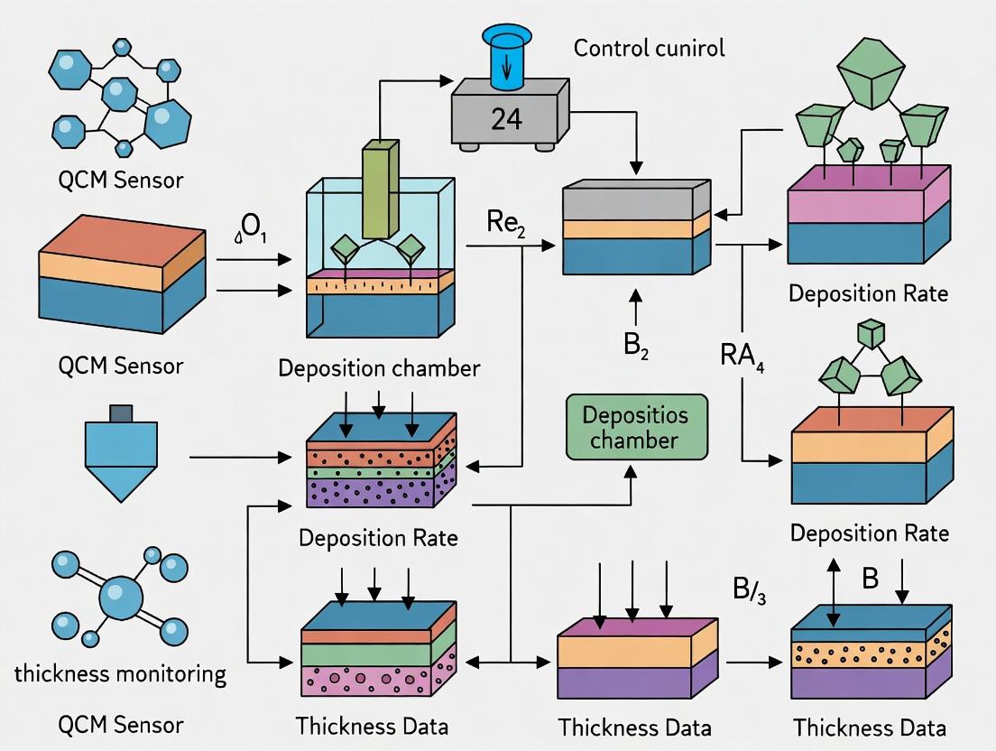
Precision Thin-Film Deposition Control: How QCM Thickness Monitoring Transforms Biomedical Device and Drug Delivery Development

Abstract

This article provides a comprehensive guide to Quartz Crystal Microbalance (QCM) thickness monitoring for precise deposition control in biomedical research and development. Targeting scientists, researchers, and drug development professionals, it explores the foundational principles of the QCM technique, details its methodological application in processes like ALD, sputtering, and organic thin-film deposition, addresses common troubleshooting and optimization challenges for accuracy, and validates its performance against alternative methods like ellipsometry and profilometry. The article synthesizes how real-time, in-situ QCM monitoring enables the reproducible fabrication of advanced drug-eluting coatings, implantable sensors, and controlled-release matrices critical to modern biomedical innovation.

The Science of Sensing: Understanding QCM Fundamentals for Deposition Monitoring

Technical Support Center: QCM Thickness Monitoring for Deposition Control

Troubleshooting Guides

Guide 1: Addressing Frequency Drift and Instability

• Issue: Unstable baseline frequency before or during deposition.
• Diagnostic Steps:
  • Verify thermal equilibration. Allow the system to stabilize for at least 30-60 minutes after reaching setpoint temperature.
  • Check for air drafts or temperature fluctuations near the measurement chamber.
  • Ensure all connections (cables, plumbing) are secure and free from mechanical stress.
  • Confirm the QCM sensor is properly seated and electrically contacted.
  • Check the quality of the vacuum or the purity/stability of the gas atmosphere in the chamber.
• Resolution Protocol: Implement a rigorous temperature control protocol and physical isolation of the setup. For vacuum systems, verify pump performance and check for leaks.

Guide 2: Incorrect or Non-Linear Mass Sensitivity

• Issue: Calculated thickness deviates from expected values based on reference measurements (e.g., ellipsometry).
• Diagnostic Steps:
  • Confirm the correct acoustic impedance (Z) and density (ρ) values for the deposited film material are entered into the model (e.g., Sauerbrey, viscoelastic model).
  • For rigid films, verify the Sauerbrey condition: ΔD dissipation shift should be < 2% of the ΔF frequency shift.
  • For soft/viscoelastic films (e.g., polymers, biomolecular layers), check if a viscoelastic model is required.
  • Ensure the deposition is uniform over the active electrode area.
• Resolution Protocol: Calibrate the QCM system using a well-characterized deposition (e.g., a known thickness of evaporated gold or silicon oxide). Switch to an extended model (e.g., Kelvin-Voigt) if dissipation changes are significant.

Guide 3: Signal Noise During Liquid-Phase Experiments

• Issue: Excessive noise when monitoring in fluid (electrolyte, buffer solutions).
• Diagnostic Steps:
  • Check for air bubbles on the sensor surface or in the flow cell. Bubbles cause massive, erratic signal shifts.
  • Verify flow stability. Peristaltic pumps can introduce pulsation-related noise.
  • Ensure the oscillator/driver circuit is properly configured for liquid-phase damping.
  • Confirm the O-ring seal is intact and not causing pressure fluctuations on the crystal.
• Resolution Protocol: Degas all buffers prior to use. Use pulse-dampeners on pump lines. Switch to a flow system with a syringe pump for smoother flow. Ensure proper O-ring seating and torque.

Frequently Asked Questions (FAQs)

Q1: Can I use the standard Sauerbrey equation for my protein adsorption experiment? A: Use the Sauerbrey equation only for an initial, approximate estimate. Protein layers are often viscoelastic. Always monitor the dissipation (D) factor simultaneously. If ΔD is substantial (>1-2% of ΔF), you must use a viscoelastic model (e.g., Kelvin-Voigt) for accurate mass determination, as the Sauerbrey equation will underestimate the wet mass.

Q2: My calculated film density seems unrealistic. What could be wrong? A: This often stems from incorrect input parameters. See Table 1 for common material properties. Double-check the assumed acoustic impedance (Z = √(ρ * μ)) of your film. For unknown materials, performing a complementary measurement (e.g., AFM on a spot sample) to determine one variable (like thickness) can help back-calculate the correct density and shear modulus.

Q3: How do I clean and reuse my QCM sensors? A: Caution: Improper cleaning destroys the electrode. A general protocol for gold sensors: 1. Rinse with appropriate solvent (e.g., ethanol, water). 2. Immerse in a gentle cleaning solution (e.g., 2% Hellmanex III, 5-10 min). 3. Rinse extensively with pure water and dry under nitrogen. 4. For organic residues, use oxygen plasma treatment (low power, <1 min). Never use strong acids (aqua regia) on patterned electrodes unless specified by the manufacturer, as they can undercut and destroy the chrome/gold adhesion layer.

Q4: What is the significance of the third harmonic in QCM data? A: The third harmonic (or other overtones, n=3, 5, 7...) provides information about the vertical structure of the adsorbed film. A uniform, rigid film will show proportional frequency shifts across all overtones (ΔF/n = constant). Discrepancies between overtones indicate a non-uniform or viscoelastic film where shear deformation decays with depth, offering insights into film softness and stratification.

Data Presentation

Table 1: Key Material Properties for QCM Modeling

Material	Density (ρ, g/cm³)	Shear Modulus (μ, GPa)	Acoustic Impedance (Z, kg/m²s)	Typical Use Case
Gold (Au)	19.3	27.0	~8.3 x 10⁶	Electrode / Reference layer
Silicon Oxide (SiO₂)	2.2-2.6	30-33	~10.0 x 10⁶	Inorganic film model
Tantalum (Ta)	16.6	69.0	~10.7 x 10⁶	Sputtering target / barrier layer
Polystyrene	1.05	~1.0	~1.0 x 10⁶	Polymer film model
Protein Layer*	~1.1-1.3	0.001-0.1	~0.04-0.4 x 10⁶	Bio-adsorption studies

*Highly viscoelastic; values are approximate and variable.

Table 2: Troubleshooting Summary: Symptoms & Likely Causes

Symptom	Likely Cause	Immediate Action
Sudden, large ΔF jump	Bubble formation/rupture	Stop flow, degas liquids, check for leaks
Gradual, continuous drift	Temperature instability	Improve thermal shielding, extend equilibration
High baseline noise	Loose connection, pump vibration	Check cables, use vibration dampeners, switch pump type
ΔF positive (increase)	Film delamination/desorption	Check film adhesion, review chemistry
ΔF & ΔD perfectly proportional (ΔD/ΔF constant)	Ideal rigid film	Sauerbrey equation is valid.

Experimental Protocols

Protocol: Calibration of QCM Mass Sensitivity via Gold Evaporation

Objective: To establish the system's mass sensitivity constant (C_f) for a rigid film.

Materials: QCM with gold-coated sensor, thermal evaporation chamber, quartz crystal monitor, thickness profiler (e.g., AFM, stylus profilometer).

Procedure:

• Record the stable baseline frequency (F0) of the clean sensor in the deposition chamber under high vacuum (<1e-6 mbar).
• Evaporate a thin layer of high-purity gold (Au) at a slow, controlled rate (~0.1 Å/s). Simultaneously monitor frequency shift (ΔF).
• Stop deposition at a target ΔF of approximately -1000 Hz.
• Vent the chamber and remove the sensor.
• Using a thickness profiler, measure the actual physical thickness (t) of the gold deposit at several points on the electrode.
• Calculate the areal mass density: Δm = ρ_Au * t (where ρ_Au = 19.3 g/cm³).
• The experimental sensitivity constant is: C_f,exp = -Δm / ΔF. Compare this to the theoretical Sauerbrey constant C_f = -n / (ρ_q * v_q), where n=1, ρq=2.648 g/cm³, vq=3340 m/s for AT-cut quartz. Agreement should be within ±5%.

Protocol: In-Situ Monitoring of Lipid Bilayer Formation (Vesicle Fusion)

Objective: To characterize the adsorption and rupture of vesicles to form a supported lipid bilayer (SLB).

Materials: QCM-D instrument, gold-coated sensor, buffer (e.g., 150 mM NaCl, 10 mM HEPES, pH 7.4), small unilamellar vesicles (SUVs, ~50 nm diameter) of desired lipid composition.

Procedure:

• Mount sensor in flow chamber. Equilibrate with >5 cell volumes of buffer at a slow flow rate (e.g., 50 µL/min) until stable F and D baselines are achieved.
• Stop flow. Inject a 0.1-0.5 mg/mL SUV suspension into the chamber. Allow to incubate without flow for 10-15 minutes.
• Observe F and D signals in real-time. Initial vesicle adsorption causes a large ΔF decrease and a large ΔD increase.
• Restart buffer flow at a higher rate (e.g., 200 µL/min) to wash away unadsorbed vesicles.
• A successful bilayer formation is indicated by a final frequency shift (ΔF_final) approximately half of the initial adsorption minimum and a dissipation shift (ΔD_final) close to zero, signifying a thin, rigid bilayer. See the diagnostic diagram below.

Mandatory Visualization

Diagram 1: QCM-D Data Interpretation Logic for Film Characterization

Diagram 2: Vesicle Fusion to Supported Bilayer Workflow

The Scientist's Toolkit: Research Reagent Solutions

Table 3: Essential Materials for QCM Bio-Sensing Experiments

Item	Function & Specification	Key Consideration
AT-cut Quartz Crystals	Piezoelectric substrate. Standard: 5 MHz, 14 mm diameter, Au electrodes.	Choose electrode material (Au, SiO₂, etc.) compatible with your surface chemistry.
Piranha Solution	(CAUTION: Extremely hazardous). For deep cleaning gold surfaces (removes organic contaminants).	Use only on plain gold chips. Never use on patterned electrodes. Proper safety gear is mandatory.
Alkanethiols (e.g., 11-MUA)	Forms self-assembled monolayers (SAMs) on gold for functionalization (COOH, OH, EG groups).	Control concentration and incubation time for a dense, ordered monolayer.
NHS/EDC Chemistry Kit	Standard carbodiimide crosslinkers for activating carboxyl groups to attach biomolecules (proteins, DNA).	Freshly prepare solutions. Optimize ratio and reaction time to minimize multi-layer formation.
Lipid Vesicles (SUVs/LUVs)	Model membrane systems for studying bilayer formation, protein-membrane interactions.	Extrude through polycarbonate membranes for uniform size. Critical for reproducible fusion.
Running Buffer Salts	Provides ionic strength and pH control (e.g., PBS, HEPES-NaCl).	Always degas/filter (0.22 µm) before QCM liquid experiments to prevent bubbles and particulates.
Viscoelastic Modeling Software	(e.g., QTools, Dfind) Analyzes ΔF/ΔD data across multiple overtones to extract film thickness, shear modulus, and density.	Essential for soft films. Requires data from at least 3 overtones for reliable fitting.

Troubleshooting & FAQ Technical Support Center

This support center is designed for researchers engaged in quartz crystal microbalance (QCM) thickness monitoring for thin-film deposition control, particularly within the context of advanced materials and drug development research.

FAQ 1: Why does my frequency shift (Δf) not correlate linearly with mass deposition during a spin-coating process, violating the Sauerbrey assumption? Answer: The Sauerbrey equation (Δm = – (C • Δf) / n) assumes a rigid, uniformly distributed mass. In spin-coating, viscoelastic, non-uniform films are common. A non-linear Δf or significant dissipation shift (ΔD) indicates a "soft" film. First, measure ΔD simultaneously. If ΔD/Δf > 1 x 10⁻⁶ Hz⁻¹, the film is viscoelastic. Use a Voigt-based model (included in most modern QCM-D software) to calculate mass. Ensure your solvent has fully evaporated, as trapped solvent dramatically alters viscoelasticity.

FAQ 2: During thermal evaporation deposition, the frequency shift becomes erratic and non-monotonic. What is the cause? Answer: This is typically a temperature effect. The QCM crystal's resonant frequency is temperature-sensitive (typically -20 to -30 ppm/°C for AT-cut crystals). High deposition rates or proximity to a hot source heats the crystal. Solution: 1) Activate the instrument's internal temperature control if available. 2) Increase the time between deposition and measurement to allow thermal equilibration. 3) Use a dual-crystal setup (one shielded from deposition) for differential thermal compensation. 4) Ensure the crystal holder is properly seated for optimal heat transfer.

FAQ 3: How do I distinguish between a true mass-loaded frequency shift and a shift caused by changes in the liquid environment's properties (e.g., buffer swap)? Answer: This is critical for biological adsorption studies. The Kanazawa-Gordon equation describes frequency dependence on liquid density (ρ) and viscosity (η): Δf ~ -n^(1/2) • (ρL • ηL)^(1/2). A buffer change alone causes a simultaneous, predictable shift in all overtones. A mass adsorption event causes a divergent shift across overtones (especially for soft films). Protocol: Always perform a stable baseline in the initial buffer prior to introduction of analyte. Use the shift from buffer A to buffer B as a system calibration for liquid property changes.

FAQ 4: My calculated film thickness from Δf deviates significantly from ellipsometry or profilometry data. Which is correct? Answer: Neither is inherently "correct"; they measure different properties. Sauerbrey-derived thickness assumes a rigid, dense film. Discrepancies arise from:

• Film porosity: QCM measures hydrated mass (including trapped solvent); ellipsometry measures optical thickness of the solid matrix.
• Film density: You must assume a density for the Sauerbrey conversion. An incorrect density assumption creates error. Troubleshooting Table:

Discrepancy	Likely Cause	Diagnostic Check	Action
QCM thickness > Ellipsometry	Porous film trapping solvent (common in biomolecular layers)	Measure in air after drying. If discrepancy reduces, porosity is confirmed.	Use QCM-D to model hydrated water content. Report both wet (QCM) and dry (ellipsometry) thickness.
QCM thickness < Ellipsometry	Assumed film density is too high, or film is viscoelastic	Check ΔD. Calculate using a viscoelastic model.	Determine the film's real density via combined QCM and X-ray reflectivity (XRR).

Experimental Protocol for Validating Sauerbrey Applicability in Deposition Control

Title: Protocol for Establishing a Sauerbrey-Based Thickness Monitor for Thermal Evaporation. Objective: To calibrate and verify a QCM sensor for accurate thickness measurement of a rigid metal film (e.g., gold) during thermal evaporation. Materials: See "Scientist's Toolkit" below. Method:

• Sensor Preparation: Clean the QCM crystal (Au-coated, 5 MHz) in a piranha solution (Caution: Highly corrosive), rinse with DI water, and dry under N₂.
• System Calibration: Place the crystal in the holder inside the deposition chamber. Pump down to high vacuum (<5 x 10⁻⁶ Torr). Record the stable baseline frequency (f₀).
• Deposition & Monitoring: Begin evaporation at a controlled, low rate (0.1 - 0.3 Å/s). Monitor Δf in real-time.
• Post-Deposition Validation: After depositing for a set time (targeting ~100 nm), stop deposition. Vent the chamber and measure the final film thickness at 3 points using a calibrated profilometer.
• Data Analysis:
  • Calculate mass load: Δm = – (C • ΣΔf) / n, where C = 17.7 ng•cm⁻²•Hz⁻¹ for a 5 MHz crystal, n=1 (fundamental).
  • Calculate QCM-derived thickness: tQCM = Δm / ρAu, assuming ρ_Au = 19.32 g/cm³.
  • Compare tQCM to the average profilometry thickness (tprof).
• Acceptance Criterion: If |tQCM – tprof| / t_prof < 5%, the Sauerbrey-based monitor is validated for this material and process.

The Scientist's Toolkit: Key Research Reagent Solutions

Item	Function & Specification	Critical Notes for Deposition Research
AT-cut Quartz Crystal	Piezoelectric sensor. Typically 5 MHz, Au electrodes.	The Sauerbrey constant (C) is crystal-specific. Note the fundamental frequency and electrode area.
QCM-D Instrument	Measures frequency (Δf) and energy dissipation (ΔD) shifts.	Essential for diagnosing viscoelasticity. Overtones (3rd, 5th, 7th) provide film homogeneity data.
Thermal Evaporation Source	Creates a vapor of the target material (e.g., Au, Al).	Deposition rate stability is key. Use a calibrated rate monitor independent of the QCM for cross-check.
Profilometer	Measures physical step height/thickness.	The gold standard for rigid film validation. Non-destructive optical profilometry is preferred.
Viscoelastic Modeling Software	Converts Δf/ΔD data to mass & thickness for soft films.	Required for polymer or biological layer analysis. Uses extended Voigt or Maxwell models.
Calibration Standard	Pre-characterized thin film (e.g., SiO₂ on Si).	Used for periodic validation of the entire measurement chain (QCM + thickness verifier).

Quantitative Data Summary: Sauerbrey Equation Parameters & Limits

Table 1: Sauerbrey Constants for Common QCM Crystals

Crystal Fundamental Frequency	Sauerbrey Constant (C)	Typical Electrode Area	Mass Sensitivity (Approx.)
5 MHz	17.7 ng•cm⁻²•Hz⁻¹	0.2 - 0.5 cm²	~0.3 ng/cm² per 0.02 Hz shift
10 MHz	4.4 ng•cm⁻²•Hz⁻¹	0.2 - 0.5 cm²	Higher resolution, more sensitive to surface roughness

Table 2: Guidelines for Sauerbrey Applicability

Condition	Sauerbrey Valid?	Alternative Model
ΔD/Δf < 1 x 10⁻⁷ Hz⁻¹ (in air/vacuum)	Yes - Rigid Film	Sauerbrey
1 x 10⁻⁷ < ΔD/Δf < 1 x 10⁻⁶ Hz⁻¹	Conditionally Valid (small error)	Sauerbrey or Light Load
ΔD/Δf > 1 x 10⁻⁶ Hz⁻¹ (in liquid)	No - Viscoelastic Film	Voigt or Kelvin-Voigt (QCM-D)
Film Thickness > ~2% of crystal thickness	No - Excessive Load	Not reliable; risk of oscillator stop.

Visualization: QCM-D Data Interpretation Workflow

Title: QCM-D Data Analysis Decision Tree

Title: Real-time Thickness Monitoring Setup

Welcome to the Technical Support Center for Quartz Crystal Microbalance (QCM) Deposition Control Research. This resource provides targeted troubleshooting and methodologies for researchers employing QCM, particularly when moving beyond Sauerbrey-based thickness calculations for viscoelastic organic layers.

Troubleshooting Guides & FAQs

Q1: My calculated film thickness from the Sauerbrey equation decreases sharply after solvent exposure, but microscopy shows the film is still present. What is happening? A: This indicates film swelling and a transition to a viscoelastic, fluid-like state. The Sauerbrey equation assumes a rigid, evenly distributed mass. A swollen, soft film does not couple fully to the crystal's shear motion, dissipating energy. The frequency shift (Δf) now has a mass-loading component and a viscoelastic component. Use the Z-Match method to decouple these.

Q2: When applying the Z-Match method, my iterative solver does not converge on a unique solution for shear modulus (G) and thickness (h). What are the common causes? A: Non-convergence often stems from:

• Poor Initial Guesses: The solver requires physically realistic starting points for G' (storage modulus) and G" (loss modulus).
• Invalid Data: The method requires simultaneous Δf and ΔD (dissipation) data. Ensure your D factor measurements are stable and calibrated.
• Excessive Noise: Low signal-to-noise ratio in ΔD, especially for thin films, makes fitting unstable. Increase deposition time or average data points.
• Model Breakdown: The film may be inhomogeneous or have a gradient in viscoelastic properties, violating the model's assumption of a uniform layer.

Q3: How do I validate that my QCM setup is accurately measuring dissipation (D) for soft films? A: Follow this calibration protocol:

• Baseline Stability: In your experimental fluid (e.g., buffer), record Δf and ΔD for at least 15 minutes. Drift in ΔD should be < 0.1 x 10⁻⁶ per minute.
• Positive Control - Rigid Film: Deposit a known, rigid material (e.g., a thin metal layer via sputtering in air). The ΔD/Δf ratio should be very small (< 1 x 10⁻⁷ Hz⁻¹).
• Positive Control - Viscoelastic Standard: Use a solution of glycerol in water (e.g., 30% w/w). Inject it and confirm a significant, stable ΔD shift accompanies the Δf shift. Compare the measured viscosity-density product to literature values.

Q4: What are the critical experimental parameters to document when reporting Z-Match-derived thickness for organic layers? A: See Table 1 for a summary of essential parameters and typical values/ranges.

Table 1: Critical Experimental Parameters for Z-Match Reporting

Parameter	Purpose/Impact	Typical Value/Range to Report
QCM Fundamental Frequency (f₀)	Determines sensitivity and penetration depth.	e.g., 5 MHz, 10 MHz
Overtone Number(s) Used	Multi-frequency data is crucial for validation.	e.g., n = 3, 5, 7 (or 1, 3, 5, 7)
Temperature	Critically affects viscosity and polymer dynamics.	e.g., 25.0 ± 0.1 °C
Solvent/Buffer Properties	Density (ρₗ) and viscosity (ηₗ) are direct model inputs.	ρₗ (kg/m³), ηₗ (Pa·s)
Film Density Assumption (ρf)	Key input for Z-Match. State how it was determined.	e.g., 1100 kg/m³ (from literature)
Initial Guesses for G' and G"	Impacts solver convergence.	e.g., G'= 10⁵ Pa, G"= 10⁴ Pa

Experimental Protocol: Z-Match Method for In-Situ Hydrogel Thickness Monitoring

Objective: To determine the swollen thickness and viscoelastic properties of a polymer hydrogel film deposited on a QCM sensor.

Materials & Reagents: See "Research Reagent Solutions" table below.

Procedure:

• QCM Preparation: Mount an AT-cut quartz crystal (e.g., 5 MHz) in the flow chamber. Establish a stable baseline in degassed PBS buffer at a controlled flow rate (e.g., 50 µL/min).
• Film Deposition: Switch flow to a solution of the polymer/precursor (e.g., 1 mg/mL chitosan in 1% acetic acid) for 10 minutes to adsorb a layer. Return to pure buffer flow for 20 minutes to wash and establish a stable Δf and ΔD for the "dry" adsorbed film.
• Solvent Exchange & Swelling: Perform a careful solvent exchange to a swelling agent (e.g., switch PBS flow to a 0.1 M NaOH solution to trigger chitosan gelation). Monitor Δf and ΔD in real-time until new stable values are reached (≥ 30 mins).
• Data Acquisition: Record Δf and ΔD for at least the 3rd, 5th, and 7th overtones throughout the experiment.
• Z-Match Analysis: a. Extract the stable Δfn and ΔDn values for the swollen film at each overtone n. b. Input known parameters: solvent density (ρₗ=1000 kg/m³), solvent viscosity (ηₗ=0.001 Pa·s), film density estimate (ρf, e.g., 1050 kg/m³). c. Use an iterative algorithm (e.g., in QTools software or a custom Python script) to solve the complex frequency shift equation for the unknown film thickness (h) and complex shear modulus (G = G' + iG''). The algorithm adjusts h, G', and G" until the calculated Δfn and ΔDn match the measured values across multiple overtones. d. Validate the solution by checking that the fitted parameters generate a curve that fits all overtone data.

Diagrams

Title: Z-Match Algorithm Iterative Workflow

Title: QCM Viscoelastic Modeling Input-Output Relationship

Research Reagent Solutions

Table 2: Essential Materials for QCM Studies of Organic Layers

Item	Function / Relevance	Example / Specification
AT-cut QCM Sensors (Gold)	Piezoelectric substrate for mass & viscoelastic sensing.	5 MHz or 10 MHz fundamental frequency, with gold electrodes.
Liquid Flow Chamber (Stopped/Flow)	Provides controlled environment for in-situ experiments.	Temperature-controlled, with low dead volume for fast exchange.
QCM-D Instrument	Measures both Frequency (Δf) and Dissipation (ΔD) shifts.	E.g., Biolin Scientific QSense or equivalent.
Viscoelastic Reference Fluids	For instrument calibration and method validation.	Aqueous Glycerol solutions (20-50% w/w) of known viscosity.
Polymer/Protein Stock Solutions	The analyte for film formation.	Prepare in appropriate buffer, filter-sterilized (0.22 µm).
Degassing Unit	Removes bubbles from eluents that cause signal noise.	In-line degasser or sonication/vacuum filtration setup.
Precision Syringe Pumps	Provides stable, pulse-free flow for kinetics studies.	Flow rate range: 1-200 µL/min.

Technical Support & Troubleshooting Center

Troubleshooting Guide

Q1: During my in-situ QCM experiment, the frequency drift is higher than expected even before deposition begins. What could be the cause and how do I resolve it? A: Excessive baseline drift (>1-2 Hz/min) often points to temperature instability. Ensure the QCM sensor and the deposition chamber have reached a complete thermal equilibrium (allow 30-60 minutes for stabilization post-vacuum/pressure change). Verify that the cooling water circulation for the QCM holder is consistent and that there are no drafts or external heat sources affecting the setup. Recalibrate the temperature compensation within the oscillator electronics if the feature is available.

Q2: The measured in-situ thickness from the QCM (using Sauerbrey) deviates significantly from my ex-situ profilometer measurement. Which one should I trust? A: This common discrepancy highlights a key advantage of in-situ data. First, confirm the Sauerbrey equation's validity (rigid, thin film in a viscous medium). If valid, trust the in-situ QCM data for the deposited mass. The ex-situ profilometer measures a physical step height, which can be affected by film density changes, solvent loss, or film relaxation after removal from the deposition environment. The QCM provides the true as-deposited mass thickness. Consider using the QCM data to calibrate your ex-situ tool for that specific material.

Q3: My in-situ QCM signal becomes noisy and unreliable when switching from a vacuum to a liquid (solvent) environment. What steps should I take? A: This is typically an oscillator/driver issue. Ensure you are using a liquid-compatible QCM sensor (sealed edge) and an oscillator/driver system designed for liquid-phase operation. Check for bubbles on the sensor surface—they cause massive damping and noise. Purge the flow cell carefully. Increase the oscillator's gain setting, if possible, to maintain stable oscillation in the higher-damping environment. Switch to a model that analyzes both frequency and dissipation (QCM-D) if the film is soft.

Q4: How do I distinguish between a genuine film deposition signal and an artifact from a changing viscosity or density of the bulk solution in my in-situ experiment? A: Monitor multiple overtones. A purely viscoelastic change in the bulk liquid will affect all overtones proportionally (Δfn / n ≈ constant). A rigid mass loading event (deposition) will show a greater frequency shift on lower overtones (Δfn / n is not constant). Running a buffer/baseline step before introducing the depositing species is critical. Using a reference crystal in a separate flow cell exposed only to the changing bulk solution can also provide a baseline for subtraction.

Frequently Asked Questions (FAQs)

Q: What is the fundamental difference between in-situ and ex-situ thickness monitoring? A: In-situ monitoring measures the film growth in real-time within the deposition environment (e.g., vacuum, liquid). Ex-situ measurement characterizes the film after processing is complete and it has been removed from its deposition environment.

Q: For drug development, what specific advantages does in-situ QCM offer in coating or layer-by-layer assembly? A: It provides real-time feedback on adsorption kinetics, revealing not just final mass but rates of binding, complex coacervation, and the conditions for self-assembly. It can monitor phase transitions, hydration, and viscoelastic properties of polymeric or biologic films, which are critical for drug delivery system stability and release profiles.

Q: Can I use the same QCM sensor for both in-situ and ex-situ measurements? A: No. Sensors used in liquid-phase or reactive environments are often sealed and may have residue. Ex-situ measurement typically requires a clean, dedicated sensor. The process of removing, cleaning, and re-mounting a sensor destroys the in-situ context and introduces uncontrolled variables.

Q: What is the typical thickness resolution of a modern research-grade in-situ QCM system? A: Modern systems can resolve mass changes down to approximately 0.5 ng/cm², which for a typical organic film density translates to a ~0.05 Å thickness resolution. This high sensitivity is unattainable with most ex-situ techniques without destructive sampling.

Q: How do I convert QCM frequency shift (ΔF) to thickness (d)? A: Use the Sauerbrey equation for rigid, thin films in air/vacuum: Δm = -C * Δf / n, where C is the sensor constant (e.g., 17.7 ng cm⁻² Hz⁻¹ for a 5 MHz AT-cut crystal), n is the overtone number. Thickness is then d = Δm / ρ, where ρ is the film density. For soft films in liquid, a viscoelastic model (e.g., Voigt) applied to multiple overtones is required.

Data Presentation: Key Performance Comparison

Table 1: Quantitative Comparison of In-Situ QCM vs. Common Ex-Situ Techniques

Feature	In-Situ QCM	Ex-Situ Profilometry	Ex-Situ Ellipsometry
Measurement Context	Real-time, in deposition environment	Post-process, ambient conditions	Post-process, ambient conditions
Primary Output	Areal mass density (ng/cm²) & viscoelasticity	Physical step height (nm)	Optical thickness & refractive index (nm)
Typical Resolution	~0.5 ng/cm² (~0.05 Å)	~0.1 nm	~0.01 nm (model-dependent)
Measurement Speed	<1 second per data point	Seconds to minutes per point	Seconds per point
Liquid Environment	Directly compatible	Not compatible (destructive)	Limited compatibility (special cells)
Film Density Assumption	Required for thickness	Not required	Required (via n)
Impact on Sample	Non-destructive	Potentially destructive (contact)	Non-destructive
Kinetic Data	Intrinsic, full trajectory	Single endpoint	Single endpoint

Table 2: Common Artifacts and Their Sources

Artifact	More Likely in In-Situ QCM	More Likely in Ex-Situ Measurement
Temperature/Pressure Drift	Yes - Critical to control	Less impactful
Film Relaxation/Swelling Change	No - Measures actual state	Yes - Removed from native environment
Ambient Contamination	No - Sealed environment	Yes - Exposure during transfer
Probe/Sensor Fouling	Yes - Can occur over long runs	Less common for single use
Model-Dependent Error	Yes (Sauerbrey vs. Viscoelastic)	Yes (Optical models for ellipsometry)

Experimental Protocols

Protocol 1: Standard In-Situ QCM Setup for Thermal Evaporation Deposition (Vacuum) Objective: To monitor the real-time growth of an organic thin film via thermal evaporation.

• Sensor Preparation: Clean a 5 MHz AT-cut gold QCM sensor in a piranha solution (3:1 H₂SO₄:H₂O₂) CAUTION: Highly corrosive, rinse with Milli-Q water, and dry under N₂ stream. Mount in a holder compatible with the deposition chamber feedthrough.
• System Baseline: Place the QCM holder in the deposition chamber, pump down to base pressure (<1 x 10⁻⁶ Torr). Allow the system to thermally equilibrate for 45 minutes with cooling water on. Record the stable frequency baseline (F₀) for at least 5 minutes.
• Deposition & Monitoring: Set the QCM electronics to record frequency (ΔF) at 1 Hz. Begin the thermal evaporation of the source material at a controlled rate (e.g., 0.1 Å/s). Monitor ΔF in real-time.
• Data Conversion: After deposition, stop the source and continue monitoring until F stabilizes. Use the Sauerbrey equation with the known sensor constant (C) and an estimated film density (ρ) to convert the total ΔF to final mass and thickness.
• Validation: After venting the chamber, measure the film thickness at a masked step using ex-situ profilometry for comparative analysis (see Protocol 2).

Protocol 2: Ex-Situ Profilometry Measurement for Cross-Validation Objective: To measure the physical step height of a film deposited on a silicon witness sample alongside the QCM sensor.

• Sample Preparation: Place a clean, masked silicon wafer near the QCM sensor during the deposition run (Protocol 1, Step 3).
• Step Creation: After deposition, carefully remove the mask using tweezers, creating a sharp film edge.
• Profilometer Setup: Calibrate the stylus profilometer using a standard step height reference. Set a scan length of 500 µm, a scan speed of 50 µm/s, and a stylus force of 1 mg.
• Measurement: Perform at least 5 scans across different areas of the step. Ensure the stylus tracks cleanly without skidding.
• Data Analysis: Use the instrument software to average the step height from all valid scans. Compare this value to the in-situ QCM-derived thickness, accounting for differences in tooling factor and actual material density.

Visualization: Experimental Workflow & Data Interpretation

Diagram 1: In-Situ vs Ex-Situ Workflow Comparison

Diagram 2: Interpreting QCM Frequency Shifts

The Scientist's Toolkit: Research Reagent & Material Solutions

Table 3: Essential Materials for QCM Thickness Monitoring Research

Item	Function & Description
AT-cut Quartz Crystals (5 MHz, Au)	The core piezoelectric sensor. Gold electrodes provide a biocompatible and functionalizable surface for adsorption studies.
QCM Liquid Flow Cell	Allows controlled introduction of liquids (buffers, analytes, polymers) to the sensor surface for in-situ monitoring of adsorption from solution.
Thermal Evaporation Source & QCM Holder	Enables in-situ monitoring of physical vapor deposition (PVD) processes. The holder incorporates cooling to prevent crystal overheating.
QCM-D Oscillator/Driver Unit	The electronics that drive the crystal oscillation and precisely measure both frequency (F) and energy dissipation (D) changes. Critical for soft film analysis.
Viscoelastic Modeling Software	Software (e.g., Dfind, QTools) that applies mechanical models (Voigt, Maxwell) to F and D data from multiple overtones to extract film thickness, shear modulus, and viscosity.
Profilometry Step Height Standard	A calibration artifact with a known, certified height (e.g., 100 nm) used to validate the accuracy of ex-situ thickness measurements.
Piranha Solution (H₂SO₄:H₂O₂)	A powerful oxidizer for rigorously cleaning gold QCM sensors to remove organic contaminants before an experiment. (Extreme Hazard).
Alkanethiols (e.g., 11-Mercaptoundecanoic acid)	A common model system for forming self-assembled monolayers (SAMs) on gold QCM sensors to test system response and create functionalized surfaces.

From Theory to Lab Bench: QCM Implementation in Biomedical Deposition Processes

Integrating QCM Sensors into PVD and Sputtering Systems for Metal and Ceramic Coatings

Technical Support Center

Troubleshooting Guides

Issue 1: Erratic or Drifting Frequency Readings During Deposition

• Q: My QCM sensor shows unstable frequency readings during sputtering, making thickness data unreliable. What could be the cause?
• A: This is often caused by temperature instability. The QCM crystal's resonant frequency is highly temperature-sensitive. Ensure active cooling of the sensor head is consistent and verify coolant lines are not kinked. Check for direct radiation heating from the plasma or target; improve shielding. Allow sufficient system and QCM temperature stabilization time (minimum 30-60 minutes) under vacuum before initiating deposition.

Issue 2: Sudden Loss of Signal or "Out of Range" Error

• Q: The QCM readout goes to zero or displays an error mid-experiment. How do I diagnose this?
• A: Follow this diagnostic flowchart:

Issue 3: Significant Discrepancy Between QCM-Measured and Profilometer Thickness

• Q: My final film thickness measured by a profilometer does not match the integrated thickness from the QCM. Why?
• A: This discrepancy is central to thesis research on deposition control. Common causes and verification protocols are summarized in the table below.

Table 1: Causes and Corrections for QCM-Profilometer Thickness Discrepancy

Cause Category	Specific Issue	Diagnostic Check	Corrective Action
Tooling Factor	Incorrect or non-uniform geometric factor.	Measure thickness at multiple substrate positions.	Re-calibrate tooling factor using a uniform, well-characterized deposition run.
Material Properties	Using default Z-factor (Acoustic Impedance) for a different material.	Compare density (ρ) and shear modulus (μ) of deposited film vs. QCM database.	Use correct, experimentally determined Z-factor for your specific film composition.
Stress & Adhesion	Film stress causing density variation or delamination.	Inspect film morphology (SEM) and adhesion (tape test).	Optimize deposition parameters (pressure, power, bias) to modify film stress state.
Sensor Condition	Excessive coating mass leading to frequency non-linearity or damping.	Check final frequency shift (Δf). Rule of thumb: Δf > 5-10% of f₀ is problematic.	Replace QCM crystal more frequently. Use a higher base frequency crystal for thicker coatings.

Frequently Asked Questions (FAQs)

Q1: How often should I replace the QCM crystal? A: Replacement is based on mass loading, not time. Adhere to the manufacturer's maximum frequency shift specification (typically 5-10% of the resonant frequency). For a 6 MHz crystal, a total Δf of -300 kHz to -600 kHz is the limit. Exceeding this causes non-linear response and eventual oscillation stop.

Q2: Can I use one QCM sensor for both metal and ceramic coatings in my thesis research? A: Yes, but the critical parameter is the correct Z-factor (acoustic impedance). You must program different material constants for each coating type. Using the Z-factor for gold while depositing Al₂O₃ will introduce large errors. Always verify with a secondary thickness measurement when changing material class.

Q3: What is the optimal placement for the QCM sensor in my sputtering system? A: Place the sensor in the same geometric plane as your substrates, at a representative location for your study (e.g., center of rotation). The key is consistency for a valid tooling factor. Shield it from direct plasma bombardment if possible. The workflow below outlines the integration and calibration process.

Q4: How do I calibrate the tooling factor for my specific setup? A: Follow this experimental protocol:

• Deposit a uniform film (e.g., Au, Si) using a simple, stable process.
• Measure the thickness (Δh) at the substrate position using a profilometer (average multiple points).
• Record the QCM integrated thickness (ΔT_QCM) for the same run.
• Calculate Tooling Factor (TF): TF = Δh / ΔT_QCM.
• Input this TF into your QCM controller's software. Re-verify with a subsequent test run.

Q5: My ceramic coating is porous. Does this affect QCM accuracy? A: Yes, significantly. The QCM measures mass per unit area, not geometric thickness. A porous film has a lower density (ρ) than a bulk, dense film. If you use the Z-factor for the bulk ceramic, the QCM will report a thickness that is less than the true geometric thickness. This is a key research area: correlating QCM mass data with film microstructure.

The Scientist's Toolkit: Essential Research Reagent Solutions

Table 2: Key Materials for QCM-Integrated PVD/Sputtering Experiments

Item	Function & Specification	Critical Note for Research
Standard Calibration Materials	High-purity (99.99%) Au or Si targets. Used for initial system and QCM tooling factor calibration.	Provides a known density and stable deposition rate baseline. Essential for thesis method validation.
QCM Crystals (AT-cut)	Typically 6 MHz, gold electrodes. The core sensor.	Keep a log of crystal usage (Δf per run). Have multiple spares. Higher freq. (e.g., 15 MHz) offer better mass resolution for thin films.
Z-Factor Reference Materials	Verified material constants (density ρ, shear modulus μ) for your specific coatings (e.g., TiN, Al₂O₃, DLC).	Do not rely on generic defaults. Source from published literature or perform own calibration. Key for accurate thickness.
Conductive Silver Paste / Vacuum Grease	For mounting crystals to sensor head, ensuring thermal and electrical contact.	Apply sparingly. Excess can outgas, contaminate the chamber, or dampen crystal oscillation.
In-situ Substrate Witness Samples	Small Si wafers or glass slides mounted near the QCM.	Provides material for post-deposition validation (profilometry, SEM, XRD) to correlate with QCM's in-situ data.
Non-contact Optical Profilometer	For post-deposition thickness validation. Must have vertical resolution < 1 nm.	The primary tool for calibrating the QCM's tooling factor and verifying Z-factor accuracy.

FAQs & Troubleshooting Guides

Q1: Our QCM sensor frequency shows an unexpected, continuous drift during the ALD purge step, not stabilizing. What could be the cause and how do we resolve it? A: This is often due to thermal disequilibrium or inadequate gas flow. The ALD reactor and QCM head must be thermally stabilized. Ensure the precursor and purge gas lines are fully purged and that the reactor is leak-tight. Implement a longer thermal soak period (e.g., 30-60 minutes) at the process temperature before initiating deposition. Verify that the QCM cooling system (if present) is operating consistently.

Q2: The calculated mass change per cycle (Δm/cycle) from QCM data is inconsistent with expected growth per cycle (GPC) from literature for our material. How should we troubleshoot this discrepancy? A: This discrepancy can arise from several factors. Follow this systematic protocol:

• Calibration Check: Verify the QCM calibration using a known standard (e.g., a calibrated mass).
• Tooling Factor: The QCM's geometric placement may sample a non-representative flux. Determine a "tooling factor" by comparing QCM-derived thickness on a witness sample to that measured by spectroscopic ellipsometry on a substrate in the primary deposition zone.
• Mass Sensitivity: Confirm the active sensor area and the validity of the Sauerbrey equation for your film stiffness. For porous or viscoelastic films, the Sauerbrey relation may overestimate mass.

Q3: We observe "QCM poisoning" where the frequency response becomes irreversible after exposure to certain precursors (e.g., TMA, metalorganics). How can we prevent or mitigate this? A: Poisoning indicates chemical reaction with the Au/Al electrodes. Use protective coatings on the QCM crystal.

• Immediate Mitigation: Increase purge times drastically to remove all precursor residues.
• Preventive Solution: Apply a thin, inert ALD coating (e.g., 5-10 cycles of Al₂O₃ using a mild oxidant like H₂O) directly onto the QCM sensor before the experiment. This protects the electrodes while allowing mass sensing.

Q4: How do we distinguish between genuine monolayer adsorption and physisorbed multilayer condensation using QCM data in ALD? A: Analyze the transient response. A true self-limiting ALD half-cycle will show a frequency shift (mass increase) that saturates exponentially within the precursor dose time and remains stable during the purge. Physisorption or condensation will show a non-saturating, linear drift during dose and/or a continued drift or decrease in mass (frequency increase) during the purge as the condensate evaporates. Implementing a variable dose-time experiment is key.

Experimental Protocol: Determining ALD Saturation Kinetics with QCM

Objective: To precisely determine the minimum precursor dose time required for saturated monolayer formation.

Materials: See "The Scientist's Toolkit" below.

Methodology:

• Setup: Load QCM sensor and substrates. Stabilize reactor at target temperature (e.g., 150°C for Al₂O₃). Establish stable N₂ purge flow.
• Baseline: Monitor QCM frequency until stable (Δf < 0.5 Hz/min).
• Saturation Experiment:
  • Fix purge and reactant (e.g., H₂O) pulse times at clearly saturating values (e.g., 0.1 s pulse, 20 s purge).
  • For the precursor (e.g., TMA), systematically vary the pulse time (tdose) across a range (e.g., 0.01, 0.02, 0.05, 0.1, 0.2, 0.5 s).
  • For each tdose, perform 1 complete ALD cycle (Precursor Dose → Purge → Reactant Dose → Purge).
  • Record the total frequency shift (Δf) for that cycle from the stable baseline before the cycle to the stable baseline after the cycle.
• Analysis: Plot Δf per cycle vs. log(tdose). The saturation point is identified as the dose time after which Δf per cycle plateaus. Data below saturation will show a steep increase in Δf with tdose.

Q5: Our QCM data is noisy, making it difficult to resolve sub-monolayer shifts (<1 Hz). What steps improve signal-to-noise? A: Sub-monolayer resolution requires exceptional stability.

• Environmental: Place the entire system on a vibration isolation table. Use a temperature-controlled lab (±0.5°C).
• Electronic: Use a high-quality, dedicated QCM controller with sub-0.1 Hz resolution. Ensure all connections are secure and shielded.
• Data Processing: Employ real-time or post-process filtering (e.g., moving average, low-pass filter) appropriate for your cycle time. Increase data sampling rate to oversample the signal.

Data Presentation

Table 1: Common ALD Processes and Typical QCM Frequency Shifts per Cycle

Material System	Precursor / Reactant	Typical Process Temp.	Expected Δf per cycle (for 5 MHz crystal)*	Saturation Dose Time (ms, typical)
Al₂O₃	TMA / H₂O	150°C	-12 to -15 Hz	50 - 100
ZnO	DEZ / H₂O	150°C	-8 to -10 Hz	100 - 200
TiO₂	TiCl₄ / H₂O	150°C	-5 to -7 Hz	100 - 200
HfO₂	TDMAHf / H₂O	250°C	-6 to -8 Hz	200 - 500
SiO₂	BTBAS / O₃	300°C	-2 to -4 Hz	500 - 1000

*Note: Δf is negative for mass increase. Exact values depend on tooling factor, crystal fundamental frequency, and process conditions.

Table 2: Troubleshooting Guide for QCM-ALD Anomalies

Symptom	Potential Cause	Diagnostic Action	Corrective Action
No frequency shift during dose	Precursor line blockage	Check precursor bubbler pressure, valve function.	Clear line, ensure bubbler has sufficient precursor.
Frequency increases (mass loss) during dose	Etching or sensor decomposition	Check process temperature compatibility with sensor.	Lower process temperature or use a protected sensor.
Non-reproducible Δf between cycles	Incomplete purging	Monitor pressure spikes during pulses.	Increase purge time or flow rate; check for dead volumes.
Sudden, permanent frequency jump	Condensation or particle drop on sensor	Inspect sensor post-run visually or with microscope.	Improve precursor vaporization; install a particulate filter.

The Scientist's Toolkit: Key Research Reagent Solutions & Materials

Item	Function in QCM-ALD Experiments
5 MHz AT-cut Quartz Crystal Microbalances (Au electrodes)	The core sensor. Au electrodes provide a conductive, clean surface for initial deposition and electrical contact.
ALD-Grade Precursors (e.g., TMA, DEZ, TiCl₄)	High-purity sources of the depositing material. Must have high vapor pressure and thermal stability for reproducible dosing.
Ultra-High Purity (UHP) Carrier/Purge Gas (N₂ or Ar)	Inert gas for transporting precursor vapors and purging the reactor between doses to prevent CVD reactions.
Inert ALD Protection Layer Precursors (e.g., H₂O for Al₂O₃)	Used to deposit a thin, protective oxide layer on the QCM sensor to prevent electrode poisoning.
Spectroscopic Ellipsometry Reference Samples	Independent, ex-situ technique for absolute thickness measurement to calibrate the QCM tooling factor.
Vibration Isolation Table	Critically dampens environmental mechanical noise to achieve sub-Hz frequency resolution.
Temperature-Controlled QCM Holder	Maintains the sensor at a stable, known temperature to minimize thermal drift during experiments.

Visualization: Experimental Workflow & Data Analysis Pathways

Monitoring Organic and Polymer Film Growth for Drug Delivery Matrices

Technical Support Center: Troubleshooting & FAQs

This support center is designed to assist researchers utilizing Quartz Crystal Microbalance (QCM) for in-situ monitoring of thin film deposition within the context of drug delivery matrix development. The guidance is framed as part of a thesis on QCM thickness monitoring for deposition control.

Frequently Asked Questions (FAQs)

Q1: My QCM frequency shift (ΔF) shows an unexpected, non-linear increase during a layer-by-layer (LbL) polymer deposition. What could be causing this? A: A non-linear, sharp increase in ΔF often indicates film instability or dissolution rather than deposition. Common causes include:

• Incorrect pH or Ionic Strength: The polymer solution's pH may be outside the stable range for complex coacervation, causing weakly adsorbed layers to desorb upon rinsing.
• Insufficient Rinsing Time: Residual salt from previous adsorption steps can interfere with subsequent layer formation, leading to inconsistent mass addition.
• Solution Degradation: Biological polymers (e.g., chitosan, alginate) may degrade if solutions are not freshly prepared or properly stored.

Q2: The calculated film thickness from the Sauerbrey equation deviates significantly from profilometer measurements. How should I resolve this? A: The Sauerbrey equation assumes a rigid, evenly distributed film. Discrepancies arise from:

• Film Viscoelasticity: Polymer/hydrogel films for drug delivery are often soft and hydrat-ed, violating the rigidity assumption. Use the QCM-D technique to monitor dissipation (ΔD).
• Liquid Trapping: Porous films trap solvent, which contributes to the measured mass but not to the dry thickness. Compare Sauerbrey thickness (wet mass) with post-drying profilometry.
• Non-Uniform Coverage: Check film morphology via AFM. The Sauerbrey equation requires uniform mass distribution across the active sensor area.

Q3: I observe significant frequency drift (>2 Hz/min) during baseline stabilization in buffer. How can I achieve a stable baseline? A: Baseline drift compromises all subsequent ΔF measurements. Troubleshoot as follows:

• Temperature Control: Ensure the measurement chamber is thermally equilibrated. Use a circulating water bath or Peltier device. Even ±0.1°C/min drift can cause significant ΔF.
• Degas Solutions: Dissolved gases in buffer can create micro-bubbles on the sensor surface. Degas all solutions under vacuum or by sonication before use.
• Secure Flow Cells: Check for leaks or pressure fluctuations in the flow system that can cause mechanical stress on the crystal.

Q4: How do I calibrate my QCM system for a non-aqueous solvent used in polymer deposition? A: The Sauerbrey constant depends on the square root of the product of crystal density and shear modulus, which can change with immersion fluid.

• Characterize the fluid's density (ρL) and viscosity (ηL).
• Establish a new baseline frequency (F0) in the static solvent.
• The mass sensitivity (C) remains ~17.7 ng/(cm²·Hz) for a 5 MHz AT-cut crystal, but the viscous damping will differ. Reference the manufacturer's guidelines for specific solvent corrections.

Troubleshooting Guides

Issue: Poor Film Adhesion and Repeatability Symptoms: Inconsistent ΔF per deposition cycle, visible delamination, or complete film loss during rinsing. Diagnostic Protocol:

• Surface Preparation: Verify sensor surface cleaning and functionalization.
  • Protocol: Sonicate sensors in 2% Hellmanex III for 15 min, rinse with water/ethanol, dry under N₂, treat with UV-Ozone for 20 min.
• Verify First Layer Attachment: Ensure the priming layer (e.g., PEI, PDA) forms a stable monolayer.
  • Protocol: Immerse clean Au sensor in 1 mg/mL polyethylenimine (PEI, pH 5.0) for 30 min. A stable ΔF shift of -25 ± 5 Hz indicates proper attachment.
• Optimize Deposition Parameters: Systematically vary contact time, concentration, and rinse time for each polymer.
  • Record parameters and resulting ΔF/cycle in a table (see below).

Issue: High Dissipation Shift Indicating Excessively Soft Films Symptoms: ΔD/ΔF ratio > 4 x 10⁻⁷ Hz⁻¹, implying a highly viscoelastic film where Sauerbrey thickness is invalid. Actionable Steps:

• Cross-linking: Introduce a mild cross-linking step (e.g., EDC/NHS for carboxy/amine groups, genipin for chitosan) to stiffen the matrix.
  • Protocol: After every 5 bilayers, expose film to 2 mL of 50 mM EDC / 25 mM NHS in MES buffer (pH 6.0) for 1 hour under stopped flow. Rinse thoroughly.
• Model with Viscoelastic Models: Use QCM-D software to fit ΔF and ΔD data to Voigt or Maxwell viscoelastic models to extract shear modulus and accurate hydrated thickness.

Data Presentation

Table 1: QCM Response for Common Drug Delivery Polymer Deposition (LbL)

Polymer Pair (Cation/Anion)	Typical Conc. (mg/mL)	Adsorption Time (min)	Avg. ΔF per Bilayer (Hz)	Avg. ΔD per Bilayer (10⁻⁶)	Sauerbrey Thickness per Bilayer (nm)	Notes
Chitosan / Alginate	1.0 / 1.0	10 / 10	-52 ± 8	3.2 ± 0.9	18.5 ± 2.8	pH 5.0 / 6.0, high viscoelasticity
Poly-L-lysine (PLL) / Hyaluronic Acid (HA)	0.5 / 0.5	5 / 5	-23 ± 3	0.8 ± 0.2	8.2 ± 1.1	pH 7.4, stable & rigid films
Polyethylenimine (PEI) / Heparin	1.0 / 1.0	15 / 15	-75 ± 12	5.5 ± 1.5	26.7 ± 4.3	For growth factor binding, very soft

Table 2: Troubleshooting Common QCM Artifacts

Artifact Symptom	Possible Root Cause	Diagnostic Check	Corrective Action
Sudden frequency spike	Air bubble on sensor	Visual inspection, unstable ΔD	Stop flow, flush chamber vigorously, degas solutions.
Gradual frequency decrease in static fluid	Contamination or bacterial growth	Check solution clarity, smell	Use sterile-filtered buffers, add 0.02% sodium azide.
No frequency change during injection	Pump failure or clogged line	Verify flow at outlet, check tubing	Prime pump, replace inlet filter, clear tubing.
Over-damped resonance	Sensor cracked or damaged	Inspect under microscope, check impedance	Replace crystal. Do not overtighten holder.

Experimental Protocols

Protocol 1: Standard QCM-D Experiment for LbL Film Growth Objective: To monitor the in-situ growth of a (PLL/HA)₁₀ multilayer film for a drug delivery matrix. Materials: See "Scientist's Toolkit" below. Method:

• Sensor Preparation: Mount a clean Au-coated QCM sensor in the flow module. Establish a stable baseline with running buffer (10 mM HEPES, 150 mM NaCl, pH 7.4) at 100 µL/min until ΔF drift < 1 Hz/min.
• Prime Layer: Inject 1 mg/mL PLL solution for 10 min (flow stopped after filling). Rinse with buffer for 15 min (flow on) to remove loosely adsorbed polymer. Record ΔF₍₁₎ and ΔD₍₁₎.
• Bilayer Deposition: Inject 1 mg/mL HA solution for 10 min (stopped flow). Rinse with buffer for 15 min. Record ΔF₍₂₎ and ΔD₍₂₎. This completes one bilayer.
• Repetition: Repeat Step 3, alternating PLL and HA solutions, until 10 bilayers are deposited.
• Data Analysis: For each bilayer, calculate the net ΔF and ΔD. Use the Sauerbrey equation (for rigid films) or viscoelastic modeling (if ΔD is significant) to calculate adsorbed mass and thickness.

Protocol 2: Post-Deposition Film Characterization (Ex-situ) Objective: To validate QCM-derived thickness and assess film morphology. Method:

• Dry Thickness Measurement: Carefully remove the sensor from the module. Use a profilometer to scratch a gentle line through the film and measure step height at 5 different points.
• Morphological Analysis (AFM): Image a 10 µm x 10 µm area of the film in tapping mode under ambient conditions. Analyze surface roughness (Ra, Rq).
• Correlation: Compare the dry profilometry thickness with the Sauerbrey thickness calculated from the final ΔF. Note: QCM reports wet mass; profilometry reports dry geometric height. A ratio (QCM/Profilometry) >1 suggests significant hydration.

Visualizations

Diagram Title: QCM-D Layer-by-Layer Deposition Workflow

Diagram Title: QCM Data Analysis Decision Tree

The Scientist's Toolkit: Research Reagent Solutions

Table 3: Essential Materials for QCM Film Growth Experiments

Item	Function / Role	Example Product & Specification
QCM-D Instrument	Core system for in-situ monitoring of frequency (ΔF) and energy dissipation (ΔD) shifts.	Biolin Scientific QSense Analyzer, or equivalent.
AT-cut Quartz Crystals	Piezoelectric sensors. Gold coating is standard for bio/polymer adsorption.	5 MHz, Au-coated (50-100 nm), diameter 14 mm.
Peristaltic or Syringe Pump	Provides precise, pulse-free flow of solutions over the sensor surface.	Ismatec IPC or Cetoni neMESYS pumps.
Polycation Solution	Provides the positively charged layer for electrostatic LbL assembly.	Chitosan (low MW, >75% deacetylated), 1 mg/mL in acetate buffer (pH 5.0).
Polyanion Solution	Provides the negatively charged layer for electrostatic LbL assembly.	Hyaluronic acid (from S. zooepidemicus), 1 mg/mL in HEPES buffer (pH 7.4).
Degassed Running Buffer	Establishes stable baseline and rinses away unbound polymer.	10 mM HEPES, 150 mM NaCl, pH 7.4, 0.22 µm filtered and degassed.
UV-Ozone Cleaner	Provides ultraclean, hydrophilic sensor surface by removing organic contaminants.	Novascan PSD Series UV-Ozone Cleaner.
Viscoelastic Modeling Software	Extracts accurate film parameters (thickness, shear modulus) from ΔF/ΔD data.	QTools, Dfind, or equivalent fitting suite.

Technical Support Center & Troubleshooting Guides

Frequently Asked Questions (FAQs)

Q1: My QCM frequency shift (ΔF) is unstable even before deposition begins. What could be the cause and how can I fix it? A: Unstable baseline ΔF is often caused by temperature fluctuations, poor crystal mounting, or electronic interference. For precise deposition endpoint research, ensure: (1) The QCM sensor is thermally equilibrated within the deposition chamber for at least 30 minutes. (2) The O-rings and crystal holder are clean and properly seated. (3) The instrument is placed away from sources of vibration or alternating magnetic fields. A stable baseline should have a ΔF drift of < ±0.5 Hz/min.

Q2: The calculated deposition rate from the QCM data disagrees with my post-deposition profilometry measurement. Which should I trust? A: Discrepancies often arise from differences in material density assumptions. The QCM uses the Sauerbrey equation (Δm = -C * ΔF/n), which assumes a rigid, uniform film with a known density. If your film is viscoelastic or porous, the QCM mass may differ from the geometric mass. Cross-validate with ellipsometry. Use the correction factors from your thesis calibration experiments.

Q3: How do I determine the correct harmonic (n) and constant (C) for my specific QCM sensor when setting a thickness endpoint? A: The fundamental constant (C) is provided by the manufacturer (typically ~17.7 ng/(cm²·Hz) for a 5 MHz AT-cut crystal). Use the 3rd or 5th harmonic (n=3 or 5) for liquid or soft film studies to minimize damping. For rigid metal or oxide depositions in vacuum, the fundamental (n=1) is often sufficient. Always document the n and C values used in your thesis methodology.

Q4: What does a sudden, large positive frequency shift during deposition indicate? A: A positive ΔF is non-physical for additive deposition and typically indicates a system error. The most common causes are: (1) Crystal Failure: The crystal has cracked or lost electrical contact. Replace the sensor. (2) Oscillator Dropout: The drive circuit can no longer sustain oscillation due to excessive damping (e.g., from a highly viscous solution). Clean the crystal and ensure the film does not exceed the dissipation (ΔD) limits.

Q5: How can I use QCM-D (with Dissipation monitoring) to improve my endpoint accuracy for soft film depositions? A: For soft, hydrated, or polymer films, monitor both ΔF and ΔD. Use the ΔD/ΔF ratio to assess film rigidity. A stable, low ΔD indicates a rigid film where the Sauerbrey equation is valid. A high or increasing ΔD signals viscoelasticity, requiring complex modeling. Set your thickness endpoint using data from the harmonic where ΔD is minimal and stable.

Experimental Protocols for Key Calibration Experiments

Protocol 1: Calibrating QCM Response Using Sputtered Gold Films Objective: To establish a correlation between QCM frequency shift and absolute film thickness for a known material.

• Setup: Load a clean QCM sensor into a calibrated sputter deposition system. Ensure the QCM is shielded from heat and plasma.
• Pre-deposition: Record baseline frequency for 5 minutes in vacuum (<1e-5 Torr).
• Deposition: Initiate Au sputtering at a constant, low power (e.g., 50W). Record ΔF in real-time.
• Termination: Stop at a target ΔF corresponding to ~100 nm theoretical thickness.
• Validation: Measure the actual film thickness at the crystal center using stylus profilometry at 5 distinct points.
• Analysis: Calculate the effective density (ρeff) from the equation: ρeff = (ΔmQCM) / (tprofilometry * A). Update the constant in your endpoint algorithm.

Protocol 2: Endpoint Determination for Organic Layer-by-Layer (LbL) Assembly Objective: To define a reproducible QCM signal endpoint for the completion of a single polyelectrolyte adsorption cycle.

• Setup: Install the QCM in a flow cell with temperature control. Use a crystal compatible with aqueous solutions.
• Baseline: Flow buffer solution until ΔF stabilizes (±2 Hz over 10 min).
• Adsorption: Introduce the polycation solution (e.g., PEI, 1 mg/mL in buffer) for exactly 10 minutes.
• Rinse: Switch to pure buffer flow until the frequency stabilizes (this is the endpoint for the first layer). Record the net ΔF.
• Repeat: Repeat steps 3-4 with the polyanion solution.
• Endpoint Logic: Define the deposition endpoint for each layer as the time when dF/dt < 0.1 Hz/sec for 60 consecutive seconds during the rinse phase.

Table 1: Common QCM Sensor Specifications and Calibration Constants

Crystal Type	Fundamental Frequency	Constant (C)	Common Application	Max. Damping (ΔD)
AT-cut, Quartz	5 MHz	17.7 ng/(cm²·Hz)	Vacuum Deposition, Rigid Films	< 1e-6
AT-cut, Quartz	5 MHz (Gold electrode)	~17.7 ng/(cm²·Hz)	Electrochemistry, Adsorption	2e-6
AT-cut, Quartz	10 MHz	4.4 ng/(cm²·Hz)	High Sensitivity Gas Sensing	< 5e-7
QCM-D Sensor	5 MHz	As calibrated	Soft Films, Polymers, Biomolecules	N/A (Monitored)

Table 2: Troubleshooting Guide: Symptoms, Causes, and Solutions

Symptom	Likely Cause	Immediate Diagnostic Action	Corrective Solution
No frequency readout	Loose cable, Dead crystal	Check electrical connections with multimeter.	Replace sensor crystal, secure all connections.
Excessive noise in ΔF signal	Vibration, EMI, Temp drift	Isolate chamber from pumps/fans. Check grounding.	Use vibration damping feet, install Faraday cage, improve temp control.
Non-linear ΔF during deposition	Film viscoelasticity, Droplet formation	Monitor ΔD (if available), inspect crystal visually post-run.	Reduce deposition rate, use a lower harmonic, ensure solvent is dry.
Frequency drift after endpoint	Temperature change, Slow film relaxation	Plot ΔF vs. √time to identify relaxation trend.	Extend stabilization time before measurement, improve thermal regulation.

The Scientist's Toolkit: Research Reagent Solutions

Item	Function in QCM Deposition Control	Example Product / Specification
AT-cut Quartz Crystals with Au Electrodes	The core piezoelectric sensor that oscillates and responds to mass changes.	5 MHz, 1-inch diameter, 100nm Au electrodes, from Inficon or Biolin Scientific.
QCM Crystal Holder (Flow Cell)	Allows for controlled liquid-phase deposition and in-situ measurements.	Teflon flow cell with Kalrez O-rings, temperature-controlled jacket.
QCM-D System with Network Analyzer	Measures both frequency (F) and dissipation (D) for soft film characterization.	QSense Analyzer (Biolin) or equivalent.
Sputter Deposition Source	For creating well-defined, uniform calibration films of known materials.	Au or SiO₂ target, 2" diameter, 99.99% purity.
Profilometer	Provides absolute thickness calibration for validating QCM mass data.	Dektak XT stylus profilometer, 1 Å height resolution.
Temperature-Controlled Chamber	Minimizes thermal drift, a major source of baseline noise in QCM signals.	Custom or OEM chamber with ±0.1°C stability.
Data Acquisition & Control Software	Enables real-time rate calculation and automated endpoint termination.	LabVIEW or Python script implementing Sauerbrey equation and derivative analysis.

Diagrams

Title: QCM Deposition Endpoint Control Workflow

Title: QCM-D Data Interpretation for Film Rigidity

Technical Support Center

Troubleshooting Guide

Q1: The QCM frequency shift is erratic and noisy during polymer (e.g., PLGA) spray-coating, making real-time thickness control impossible. What could be the cause? A: Erratic frequency shifts are often due to droplet impact effects and inconsistent mass loading. This is not a true mass change but an artifact. Ensure the spray nozzle is precisely aligned, the carrier gas pressure is stable (e.g., 20 psi ± 0.5 psi), and the QCM sensor is placed at an optimal distance (typically 10-15 cm) and angle (90°) to the spray plume. Implement a pulsed spray with "off" periods (e.g., 10 sec spray, 30 sec pause) to allow frequency stabilization and data recording. A solvent trap and temperature stabilization chamber around the QCM are also recommended.

Q2: After depositing the drug layer (e.g., Sirolimus), the QCM shows a mass decrease over time instead of stabilization. What does this indicate? A: A continuous mass decrease indicates sublimation or desorption of the crystalline drug film under vacuum or ambient conditions. This is a critical issue for accurate mass/ thickness calibration. Verify the QCM chamber is sealed and maintained at a stable, controlled temperature (e.g., 20°C). For volatile drugs, consider a very rapid transition to the subsequent capping layer deposition to minimize exposure. Calibrate the frequency-to-mass conversion for the specific drug using an independent method (e.g., profilometry on a test substrate) to establish a corrected sensitivity factor.

Q3: The final drug release profile in PBS (pH 7.4, 37°C) shows a large initial burst release (>40% in 24 hours) instead of the desired sustained release. What fabrication parameter likely failed? A: A large burst release typically indicates a defective or discontinuous topcoat barrier layer. This can result from insufficient topcoat thickness or solvent-induced damage during deposition. Troubleshoot by: 1) Verifying the QCM-measured topcoat thickness meets the target (e.g., >2 µm). 2) Confirming the spray solvent for the topcoat does not dissolve the underlying drug layer (use orthogonal solvents). 3) Performing SEM cross-section analysis to check for pinholes or cracks in the barrier layer.

Q4: The adhesion of the multilayer coating to the stent substrate fails during expansion in a stent expansion test. How can the process be improved? A: Adhesion failure often originates at the substrate-polymer interface. Ensure the stent substrate (e.g., 316L stainless steel or CoCr alloy) undergoes rigorous pre-cleaning (sequential ultrasonic baths in acetone, isopropanol, and deionized water) and plasma activation (e.g., O2 plasma, 100 W, 2 minutes) immediately before the primer layer deposition. Verify the primer layer (e.g., a thin, adhesive polymer like parylene-C or a silane) is applied uniformly and its thickness (monitored by QCM) is within the optimal range (50-150 nm).

Frequently Asked Questions (FAQs)

Q: What is the typical frequency shift range I should expect for a 1 µm thick PLGA coating on a standard 5 MHz QCM sensor? A: Using the Sauerbrey equation (Δm = -C * Δf, where C ≈ 17.7 ng/(cm²·Hz) for a 5 MHz AT-cut crystal), a 1 µm thick PLGA film (density ~1.3 g/cm³) would cause a frequency shift of approximately -7350 Hz. Significant deviation may indicate non-rigid film behavior.

Q: Can QCM differentiate between the mass of the polymer and the encapsulated drug in a co-sprayed mixture? A: No, QCM measures the total areal mass (ng/cm²) deposited. It cannot distinguish between individual components in a blended film. To control individual layer thickness, use a sequential layered deposition approach (primer -> drug -> polymer barrier).

Q: How do I convert QCM frequency data to a physical thickness for my coating? A: You require the film's density (ρ). The basic conversion is: Thickness (cm) = Δm / ρ, where Δm is the mass change from QCM. Determine ρ independently (e.g., by measuring mass and volume of a freestanding film). For dense films, use: d (µm) = |Δf (Hz)| / [k * f₀² (MHz)], where k is a material constant (~0.0177 for PLGA).

Q: What is the most critical QCM parameter to monitor for process reproducibility? A: The Dissipation Factor (D) is critical for soft, viscoelastic polymer/drug films. A stable, low ΔD/Δf ratio indicates a rigid, well-formed film suitable for Sauerbrey analysis. A high or changing ratio signals a poorly structured, hydrating, or dissolving layer that complicates thickness interpretation.

Table 1: Target Coating Architecture & QCM Parameters

Layer	Material Example	Target Thickness (µm)	Target QCM Frequency Shift (Hz)*	Key Function
Primer	Parylene-C	0.1	-700	Adhesion promotion
Drug	Sirolimus (Crystalline)	3.0	-22,000	Therapeutic agent
Barrier	PLGA (50:50)	5.0	-36,750	Control drug release rate

*Calculated for a 5 MHz sensor with assumed densities: Parylene-C (1.1 g/cm³), Sirolimus (1.1 g/cm³), PLGA (1.3 g/cm³).

Table 2: Common QCM Troubleshooting Signals & Interpretations

Observed Signal	Probable Cause	Corrective Action
Δf oscillates wildly during spray	Droplet impact artifact	Use pulsed spray; increase nozzle-to-sensor distance.
Steady Δf decrease post-deposition	Film instability/drug sublimation	Improve environmental control; seal chamber.
High Dissipation (ΔD) increase	Film swelling or softening	Verify solvent has fully evaporated; check temperature.
Non-linear Δf during deposition	Change in film viscoelasticity	Switch to a model for soft films (e.g., Voigt).

Experimental Protocols

Protocol 1: Sequential Spray-Coating with QCM Monitoring

• Substrate Preparation: Mount a clean QCM sensor in the coating chamber. Record baseline frequency (f₀) and dissipation (D₀) in air.
• Primer Deposition: Spray the primer solution (e.g., 0.5% w/v Parylene-C in dichloromethane) using a pulsed spray cycle (1 sec spray, 10 sec pause). Monitor Δf until the target shift (-700 Hz) is reached. Cure under vacuum for 1 hour.
• Drug Layer Deposition: Spray the drug solution (e.g., 2% w/v Sirolimus in acetone/ethanol). Use a fine mist setting. Pause frequently to allow solvent evaporation and stable frequency reading. Stop at target Δf (-22,000 Hz).
• Barrier Layer Deposition: Immediately spray the polymer solution (e.g., 5% w/v PLGA in chloroform). Monitor Δf and ΔD. A low ΔD/Δf ratio confirms a rigid film. Stop at target Δf (-36,750 Hz).
• Curing: Place the coated sensor in a vacuum desiccator for 24 hours to remove residual solvents.

Protocol 2: In-Vitro Drug Release Profiling (USP IV Flow-Through Cell)

• Sample Preparation: Fabricate coated stents or representative coated substrates (e.g., coupons). Accurately weigh each sample (M_total).
• Setup: Place each sample in a flow-through cell. Use Phosphate Buffered Saline (PBS, pH 7.4) as release medium, maintained at 37°C. Set flow rate to 10 mL/hour.
• Sampling: Collect eluent fractions at predetermined time points (e.g., 1, 2, 4, 8, 24, 72, 168 hours).
• Analysis: Quantify drug concentration in each fraction using HPLC-UV. Calculate cumulative drug release as a percentage of total drug mass (M_drug, determined from QCM data or separate validation).
• Modeling: Fit release data to kinetic models (e.g., Higuchi, Korsmeyer-Peppas) to characterize release mechanisms.

Diagrams

Title: QCM-Controlled Sequential Spray Coating Workflow

Title: Troubleshooting Drug Release Profile Failures

The Scientist's Toolkit: Research Reagent Solutions

Table 3: Essential Materials for Stent Coating Fabrication & Analysis

Item	Function & Key Detail
5 MHz Gold-Coated QCM Sensors	Core tool for in-situ areal mass deposition monitoring. Gold surface allows for good adhesion of organic layers.
Precision Ultrasonic Spray Coater	Enables uniform, controlled layer deposition on small, complex stent geometries.
Poly(D,L-lactide-co-glycolide) (PLGA 50:50)	Biodegradable polymer for the barrier layer. 50:50 lactide:glycolide ratio offers moderate degradation rate (~1-2 months).
Sirolimus (Rapamycin) - USP Grade	Model anti-proliferative drug. Low solubility in water enables sustained release kinetics.
Parylene-C Dimer	Vapor-deposited or sprayable primer for exceptional adhesion to metallic substrates and drug/polymer layers.
Phosphate Buffered Saline (PBS), pH 7.4	Standard physiological medium for in-vitro drug release studies. Must contain 0.01% w/v sodium azide to prevent microbial growth.
HPLC-UV System with C18 Column	Essential analytical tool for quantifying drug concentration in release studies. Validated method required for Sirolimus.
Scanning Electron Microscope (SEM)	For critical point inspection of coating morphology, layer continuity, and cross-sectional thickness validation.

Maximizing Accuracy: Troubleshooting Common QCM Challenges in Deposition Control

Identifying and Mitigating Temperature and Stress Effects on Crystal Frequency

Technical Support Center: Troubleshooting & FAQs

FAQ 1: Why does my Quartz Crystal Microbalance (QCM) resonance frequency drift unpredictably during a long-term deposition experiment? Answer: Unpredictable drift is often caused by inadequate temperature stabilization. The quartz crystal's resonant frequency is highly sensitive to ambient temperature changes due to the temperature coefficient of the crystal cut (e.g., AT-cut). Even fluctuations of ±0.1°C can cause measurable frequency shifts that obscure mass deposition data. Ensure your deposition chamber and crystal holder are within a temperature-stabilized enclosure, and allow sufficient time for thermal equilibrium before beginning deposition.

FAQ 2: How can I distinguish between frequency shifts caused by film stress and those caused by actual mass deposition? Answer: Stress effects from the deposited film manifest as non-linear frequency changes and can cause hysteresis upon cooling or post-deposition. To distinguish, monitor the dissipation factor (D) in a QCM-D system. A pure mass load typically shows a proportional change in f and D. A significant stress effect may cause a disproportionate D shift or a frequency shift in the opposite direction to that expected from mass addition. Conducting post-deposition thermal cycling can also reveal stress-related frequency shifts.

FAQ 3: What is the best practice for mounting the crystal to minimize mounting stress effects? Answer: Use a manufacturer-recommended holder and mounting clips. Apply only the minimal torque necessary to establish good electrical contact. Over-tightening can induce static stress, altering the baseline frequency. Utilize crystals with standardized electrode pads and holders designed for uniform pressure distribution. Before any experiment, record a baseline frequency spectrum in air; excessive broadening of the resonance peak can indicate mounting stress.

Experimental Protocol: Characterizing Temperature Coefficient of Frequency (TCF)

• Setup: Place the QCM sensor in an environmental chamber with precise temperature control (±0.01°C). Connect to a high-resolution impedance analyzer.
• Stabilization: Set the chamber to a starting temperature (e.g., 20°C) and stabilize for 30 minutes.
• Measurement: Record the fundamental resonant frequency (f0).
• Ramping: Incrementally increase the temperature in steps (e.g., 1°C steps from 20°C to 40°C). Allow 15 minutes of stabilization at each step before recording f0.
• Analysis: Plot f0 vs. Temperature. The slope of the linear fit region is the TCF (Hz/°C). This value is critical for compensation algorithms.

Experimental Protocol: Assessing Film Stress via Post-Deposition Thermal Cycling

• Deposit: Perform your standard thin-film deposition on the QCM crystal under controlled conditions.
• Initial Read: Record frequency (fpost) and dissipation at experiment temperature (Texp).
• Cycle: Place the coated crystal in a thermal stage. Cycle the temperature: Texp → Texp - 10°C → Texp + 10°C → Texp.
• Monitor: Measure frequency at each stabilized temperature point and upon return to T_exp.
• Interpretation: A frequency that does not return to f_post indicates stress relief or viscoelastic changes in the film. The hysteresis loop area quantifies stress-related energy loss.

Quantitative Data Summary

Table 1: Typical Temperature Coefficients for Common Quartz Cuts

Crystal Cut	Optimal Angle	Primary Use	Temperature Coefficient (Typical, near 25°C)
AT-Cut	35°15'	Thin-film monitoring	~0 ± 1 ppm/°C
SC-Cut	34°-35°	High-stability sensors	~0 ± 0.5 ppm/°C
IT-Cut	~-19°	Wide-temperature range	~-20 ppm/°C

Table 2: Troubleshooting Frequency Instability

Symptom	Possible Cause	Diagnostic Check	Mitigation Action
Slow, unidirectional drift	Temperature drift in lab	Log ambient temperature at sensor	Use an active temperature-controlled holder
Sudden frequency jump	Mounting stress shift or particle impact	Inspect mounting clips; check for dust	Re-mount crystal with calibrated torque; clean environment
Noisy, erratic signal	Poor electrical contact or interference	Check contact springs/electrodes	Clean electrode contacts; use shielded cables
Frequency shift opposes mass load prediction	Dominant film stress effect	Perform in-situ D measurement	Modify deposition parameters (rate, power) to reduce stress

Research Reagent Solutions & Essential Materials

Table 3: Key Materials for QCM Stress & Temperature Studies

Item	Function	Example/Note
AT-cut Quartz Crystals (Gold Electrodes)	Primary sensor for mass deposition. AT-cut offers minimal TCF near room temp.	5 MHz or 10 MHz, diameter matched to holder.
Temperature-Controlled Crystal Holder	Maintains sensor at constant T, nullifying ambient fluctuations.	Must have direct temperature feedback and Peltier control.
High-Resolution Impedance Analyzer / QCM-D System	Accurately measures resonance frequency (f) and dissipation (D) shifts.	Enables stress vs. mass load discrimination.
Standardized Cleaning Solutions	Ensures reproducible surface conditions.	Piranha solution (Caution: Reactive), UV-Ozone cleaner, ethanol.
Calibrated Torque Screwdriver	Applies consistent, minimal force during crystal mounting.	Prevents mounting stress induction. Typically 2-4 cN·m.
Reference Material for Deposition (e.g., TiO2, Al2O3)	Well-characterized film for system validation.	Used to benchmark stress behavior and TCF compensation.

Visualization: QCM Frequency Shift Decision Pathway

Diagram Title: Decision Tree for Diagnosing QCM Frequency Shifts

Visualization: Experimental Workflow for Stress/TCF Analysis

Diagram Title: Workflow for Isolating Mass, Stress, and Temperature Effects

Addressing Acoustic Impedance Mismatch in Multi-Layer and Liquid-Phase Deposition

Technical Support Center

Troubleshooting Guides & FAQs

Q1: During a layer-by-layer polymer deposition in an aqueous environment, our Quartz Crystal Microbalance (QCM) frequency shifts become erratic and non-linear after the third layer. What is the likely cause and solution?

A: The likely cause is a significant acoustic impedance mismatch between the successively deposited polymer layers and the liquid medium. As the film grows, its composite acoustic impedance diverges from that of the quartz sensor and the bulk liquid, violating the Sauerbrey condition. Energy is lost into the liquid, dampening the oscillation.

Protocol for Diagnosis & Correction:

• Monitor Dissipation (D): Always use a QCM-D instrument. A continuous increase in dissipation factor (ΔD) with each layer confirms viscoelastic loading and acoustic decoupling.
• Model the Data: Use a viscoelastic model (e.g., Kelvin-Voigt) in your QCM-D software, inputting estimated densities for each polymer layer. Do not rely on the Sauerbrey equation.
• Protocol Adjustment: Introduce an intermediate drying step (gentle N₂ stream) after every 2-3 layers. Measure frequency in air to establish a stable Sauerbrey-valid baseline, then rehydrate. This resets the acoustic interface.
• Verification: Confirm film thickness and uniformity with an independent method like ellipsometry or AFM on a companion substrate.

Q2: We observe negative frequency shifts upon adsorption of protein from a high-viscosity, glycerol-containing buffer. Does this mean mass is being removed?

A: No. This is a classic artifact of an acoustic impedance mismatch between the bulk liquid and the sensor-loaded film. A high-viscosity liquid has a high acoustic impedance. When a rigid protein film (with a different impedance) adsorbs, it can alter the overall coupling of the sensor to the liquid bulk, sometimes resulting in an apparent negative ΔF. The key is the concurrent dissipation shift.

Diagnostic Protocol:

• Check ΔD: A negative ΔF with a large increase in ΔD strongly indicates a liquid property-dominated artifact.
• Perform a Buffer Baseline: Ensure the crystal is equilibrated in the high-viscosity buffer until ΔF and ΔD are perfectly stable before injecting protein. Any drift invalidates the measurement.
• Dilution Series: Repeat the experiment with a series of buffer viscosities (e.g., 0%, 5%, 10% glycerol). Plot ΔF vs. viscosity for the same protein mass. A non-linear or inverted trend confirms impedance mismatch interference.
• Solution: Switch to a lower-viscosity buffer if biologically permissible. Alternatively, use the QCM-D data at multiple overtones to fit an acoustic multilayer model that accounts for the liquid properties.

Q3: For metal-organic framework (MOF) deposition from solution, how do we differentiate between mass uptake and solvent trapping in the pores using QCM?

A: Solvent trapping (hydrodynamic coupling) presents as an acoustic impedance mismatch issue, where the trapped liquid oscillates with the MOF film, appearing as added mass. The solution lies in comparing responses in different solvents.

Experimental Protocol:

• In-Situ Deposition: Monitor MOF growth in the synthesis solution (Solution A).
• Solvent Exchange: Stop the reaction. Carefully exchange the mother liquor for a pure, miscible solvent (Solvent B) with different density (ρ) and viscosity (η). Use slow, low-shear flow.
• Measure Frequency Shift (ΔF_exchange): The ΔF observed upon exchange is directly related to the mass of trapped solvent within the MOF pores that was replaced.
• Calculate Dry Mass:
  • The frequency in Solvent B (F_B) reflects the mass of the dry MOF framework plus the mass of trapped Solvent B.
  • The true dry mass can be estimated by applying a correction factor derived from the Kanazawa-Gordon equation for the two different liquids. The change in dissipation (ΔD) during exchange is critical for this model.

Table 1: Acoustic Impedance (Z) of Common Materials in QCM Experiments

Material	Acoustic Impedance (Z) [10⁶ kg m⁻² s⁻¹]	Notes for QCM
Quartz (AT-cut)	8.84	Reference sensor material.
Water (25°C)	1.48	Standard liquid-phase reference.
Phosphate Buffered Saline (PBS)	~1.50	Similar to water.
30% Glycerol/Water	~2.15	High Z can cause mismatch artifacts.
Polyethyleneimine (PEI) wet film	~2.0 - 3.5	Depends on hydration; viscoelastic.
Polystyrene (rigid)	~2.5	Close to quartz, good coupling.
Gold (electrode)	62.1	Very high Z, thin layer assumed.
Typical Protein Film (hydrated)	~1.8 - 2.3	Property varies with conformation.

Table 2: Troubleshooting Symptoms vs. Likely Causes

Observed Symptom (in Liquid)	Concomitant Damping (ΔD)	Likely Primary Cause	Recommended Action
Non-linear ΔF vs. time/added layer	Continuously increasing	Film Viscoelasticity / Impedance Mismatch	Use viscoelastic modeling; add drying steps.
Negative frequency shift (ΔF)	Large increase	Liquid Property Interference	Verify buffer baseline; reduce viscosity.
Frequency drift never stabilizes	Drift mirrors ΔF	Temperature or flow rate instability	Thermostat cell ±0.05°C; calibrate pump.
Step-like ΔF jumps, then reversals	Erratic	Non-specific binding or film swelling	Improve surface passivation; check pH/ionic strength.
Overtone dependence diverges	High & variable	Soft, water-rich adsorbed layer	Analyze multiple overtones with appropriate model.

Experimental Protocols

Protocol: Validating the Sauerbrey Condition in Multi-Layer Deposition Objective: To determine the point at which a growing multi-layer film transitions from rigid (Sauerbrey-valid) to viscoelastic (requires modeling). Materials: QCM-D with flow cell, polymer solutions A & B, buffer, N₂ gas source. Procedure:

• Baseline: Establish stable ΔF & ΔD in buffer at 25°C.
• Layer 1 Adsorption: Introduce polymer A solution for 10 min.
• Rinse: Switch to buffer. Record final ΔF₁ and ΔD₁.
• Layer 2 Adsorption: Introduce polymer B solution. Rinse. Record ΔF₂, ΔD₂.
• Repeat for n layers.
• Drying Step: After layer n, stop flow. Gently dry the crystal and cell with a stream of N₂ until frequency stabilizes (dry film mass, Sauerbrey valid).
• Rehydration: Reintroduce buffer slowly. Record the stable ΔFhyd and ΔDhyd.
• Analysis: Plot ΔF (dry) vs. layer number. It should be linear. Plot ΔD (hydrated) vs. layer number. A sharp increase indicates the onset of significant impedance mismatch/softening. The hydrated ΔF will deviate from the dry ΔF trend after this point.

Protocol: Solvent Trapping Correction for Porous Film Mass Determination Objective: To deconvolute the dry mass of a porous film from the mass of trapped solvent. Materials: QCM-D, MOF synthesis solution (Solvent A: e.g., water/DMF), pure exchange solvent (Solvent B: e.g., ethanol), syringe pump. Procedure:

• Deposition: Synthesize/MOF deposit onto sensor from Solvent A until film growth completes. Record final ΔFA and ΔDA.
• Stabilization: Rinse with excess Solvent A to remove unreacted precursors. Stabilize signal.
• Solvent Exchange: Initiate a very slow flow (e.g., 10 µL/min) of Solvent B. Monitor ΔF and ΔD in real-time.
• Equilibration: Continue exchange until a new stable frequency (ΔFB) and dissipation (ΔDB) are reached. This may take hours.
• Calculation:
  • The measured ΔFA is proportional to (MassMOF + MassTrappedA).
  • The measured ΔFB is proportional to (MassMOF + MassTrappedB).
  • The ΔFshift (ΔFB - ΔFA) is proportional to (MassTrappedB - MassTrappedA).
  • Using the known densities and viscosities of Solvents A & B, apply a viscoelastic or acoustic layer model that includes liquid properties to solve for the dry MassMOF.

Visualizations

Title: QCM Data Analysis Decision Tree for Impedance Issues

Title: Diagnosing Negative Frequency Shift Artifacts

The Scientist's Toolkit: Research Reagent Solutions

Table 3: Essential Materials for QCM Impedance Mismatch Studies

Item	Function & Relevance to Impedance Mismatch
QCM-D Instrument	Essential for measuring energy dissipation (D). The key parameter for detecting soft films and acoustic decoupling caused by impedance mismatch.
Viscoelastic Modeling Software (e.g., QSense Dfind, QTools)	Software that uses ΔF & ΔD at multiple overtones to model film thickness, shear modulus, and density, correcting for mismatch.
Gold-coated QCM Sensors (AT-cut)	Standard sensors. Clean, flat gold surfaces are crucial for reproducible film formation and modeling.
Piranha Solution (or UV-Ozone Cleaner)	For radical cleaning of sensor surfaces. Contaminants cause uneven deposition and unpredictable acoustic coupling.
Alkanethiol Self-Assembled Monolayer (SAM) Kits	To create well-defined, rigid hydrophobic or hydrophilic surfaces as a foundation for deposition, simplifying initial acoustic conditions.
Precise Density Meter / Viscometer	To accurately characterize the density and viscosity of liquid samples. These values are direct inputs for acoustic models (Kanazawa equation).
Controlled Environment Chamber	Temperature fluctuations change liquid density/viscosity and film properties, creating drift and artifacts that mimic impedance issues.
Ellipsometer or AFM	For independent, ex-situ measurement of film thickness and morphology. Critical for validating QCM models and confirming predictions.

Sensor Contamination, Cleaning Protocols, and Crystal Lifetime Management

Technical Support Center & FAQs

Q1: What are the most common signs of QCM sensor contamination during a deposition experiment, and how do they differ from normal frequency shifts? A: Contamination manifests as anomalous, non-reproducible changes in frequency (Δf) and dissipation (ΔD). Key indicators include:

• An irreversible frequency drop after venting the deposition chamber, indicating adsorption of atmospheric contaminants.
• A continuous baseline drift (>1 Hz/hour under stable vacuum/conditions) not attributable to temperature fluctuations.
• A significant, permanent shift in harmonic overtones relative to the fundamental frequency, suggesting a non-rigid, viscoelastic layer.
• Increased noise (jitter) in the frequency signal.

Normal deposition shifts are reproducible, stable under constant conditions, and show overtone behavior consistent with a rigid film (overtones scaling proportionally).

Q2: What is the recommended protocol for cleaning a gold-coated QCM sensor contaminated with organic residues from a biofouling experiment? A: Follow this sequential, escalating-cleaning methodology. Always handle crystals with gloves and tweezers.

Step	Reagent/Solution	Procedure	Duration	Purpose	Caution
1	Hellmanex III (2%) or Alconox (1%)	Gentle sonication in warm (< 50°C) solution.	10-15 min	Removes soluble organic and ionic contaminants.	Do not scratch the electrode.
2	Deionized Water	Rinse thoroughly under a gentle stream, then sonicate in fresh DI water.	2x 5 min rinse/sonicate	Removes all traces of detergent.
3	Absolute Ethanol or Isopropanol	Sonicate in solvent.	10 min	Removes hydrophobic organics and promotes drying.	Use HPLC grade.
4	piranha solution(3:1 v/v Conc. H₂SO₄ : H₂O₂)	EXTREME CAUTION. Immerse crystal.	30-60 sec max	Removes tenacious organic and carbonaceous residues.	Highly corrosive & exothermic. For gold electrodes only. Do not use on patterned or silver electrodes.
5	Deionized Water	Immediate and copious rinsing after piranha.	>2 min rinse	Quenches and removes piranha solution.
6	Nitrogen Stream	Dry the crystal with a gentle stream of clean, dry N₂.	Until dry	Prevents water spots and streaks.

Q3: How can I extend the operational lifetime of my QCM crystals, especially in aggressive chemical or plasma environments? A: Lifetime management involves proactive protection and monitoring.

Strategy	Action	Rationale
In-situ Protection	Use a sacrificial shield or cooled crystal holder in plasma systems.	Minimizes direct ion bombardment and heat load on the active electrode.
Chemical Compatibility	Verify solvent compatibility with electrode material (e.g., no halides on silver).	Prevents irreversible electrode corrosion and delamination.
Calibration Check	Perform a periodic baseline check in a clean, dry N₂ atmosphere.	Monitors for permanent frequency shift indicating mass gain/loss from fatigue or coating damage.
Handling & Storage	Store in a dry, clean environment (e.g., nitrogen box or desiccator).	Prevents atmospheric adsorption and oxidation before use.
Stress Monitoring	Regularly monitor the motional resistance (R) or dissipation (D).	A sustained increase indicates increased viscoelastic damping, potentially from subsurface cracks or delamination.

Q4: Our research involves monitoring the adsorption of protein-drug complexes. How do we distinguish between specific binding signals and non-specific contamination? A: This requires controlled reference experiments. The workflow below details the necessary parallel experiments and data analysis steps to deconvolute the signals.

Title: Experimental Workflow to Isolate Specific Binding Signal in QCM

Q5: Can you provide a quantitative guideline for acceptable vs. critical frequency drift rates for a 5 MHz AT-cut crystal in vacuum? A: Yes. Acceptable drift is dependent on the required resolution of your deposition experiment. Below is a general guideline.

Stability Class	Drift Rate (Hz/hour)	Typical Cause	Action Required
Excellent	< 0.5	Intrinsic crystal noise, superb vacuum/temperature stability.	None. Ideal for sub-monolayer deposition studies.
Acceptable	0.5 - 2.0	Minor temperature variation, very slow outgassing/contamination.	Verify temperature control. May require baseline subtraction for long runs.
Concerning	2.0 - 5.0	Significant temperature drift, early-stage contamination, poor vacuum.	Investigate and correct environmental controls. Clean sensor.
Critical / Unstable	> 5.0	Active contamination (e.g., oil backstreaming), severe temperature change, sensor damage.	Stop experiment. Identify and eliminate contamination source. Clean or replace sensor.

---

The Scientist's Toolkit: Research Reagent Solutions

Item	Function in QCM Research
Hellmanex III or Alconox	Alkaline, surfactant-based laboratory detergents for initial, gentle removal of organic and biological residues from sensor surfaces.
Piranha Solution (H₂SO₄:H₂O₂)	A powerful, aggressive oxidizing solution for stripping tenacious organic contaminants from gold electrodes. Handle with extreme care.
UV-Ozone Cleaner	A less-harsh alternative to piranha. Uses UV-generated ozone to oxidize and remove thin organic adlayers, ideal for pre-cleaning before functionalization.
Plasma Cleaner (Ar/O₂)	Provides a dry, energetic cleaning method via ion bombardment and radical oxidation. Effective for removing hydrocarbons and activating surfaces.
11-Mercaptoundecanoic Acid (11-MUA)	A thiol-based self-assembled monolayer (SAM) molecule used to functionalize gold sensors with a carboxyl-terminated surface for biomolecule immobilization.
N-Hydroxysuccinimide (NHS) / 1-Ethyl-3-(3-dimethylaminopropyl)carbodiimide (EDC)	Crosslinking chemistry reagents used to activate carboxyl groups (e.g., on an 11-MUA SAM) for covalent coupling of amine-containing ligands (proteins, antibodies).
Bovine Serum Albumin (BSA)	A common protein used to create non-functional, passivated control surfaces to block non-specific binding in bio-sensing experiments.
Temperature-Controlled Crystal Holder	A critical peripheral to maintain the QCM sensor at a constant, known temperature, minimizing thermal drift which mimics mass-loading signals.

Troubleshooting Guides & FAQs

Q1: My QCM frequency shift during a known density material calibration is significantly lower than expected. What could be the cause? A: This typically indicates a mass loading error. First, verify the material's density and deposition rate. Ensure the QCM crystal surface is clean and the oscillator circuit is locked. Check for temperature deviations; even a 1°C shift can impact frequency. Confirm the tooling factor is correctly entered into the controller software. If the issue persists, perform a crystal impedance analysis to check for viscoelastic effects, which are unlikely with solid metals but possible with improper calibration layers.

Q2: During system verification, the measured thickness from the QCM deviates from the profilometer measurement. Which value should I trust? A: Do not automatically trust either. This discrepancy is the core of verification. Follow this protocol: 1) Measure the calibration film with a profilometer at 5+ points across the deposition zone to establish a reference mean thickness and standard deviation. 2) Compare the QCM's integrated thickness reading. A consistent, fixed offset suggests a tooling factor error. A non-linear deviation may indicate a rate-dependent error in the QCM's calibration or stress-related frequency changes. Re-calibrate using the known density material, ensuring the deposition rate matches your experimental conditions.

Q3: After changing the QCM crystal, my density calibration seems off. What steps must I be taken? A: Crystal replacement requires a full recalibration sequence. 1) Install the new crystal and perform a in-situ cleaning cycle (e.g., Ar plasma if compatible). 2) Run a baseline stability test in vacuum or process gas for 30 minutes. Frequency drift should be < 0.5 Hz/min. 3) Deposit a known density material (e.g., Al, Ag) at a low, controlled rate (0.1-0.3 nm/s). 4) Use the profilometer-measured thickness to back-calculate and update the tooling factor for that specific crystal in your software.

Q4: How often should I verify my QCM system with known density materials? A: The verification schedule depends on usage:

• Before a critical series of experiments: Always.
• After any maintenance: Including venting the chamber, replacing sources, or cleaning shutters.
• After crystal replacement: Mandatory.
• Routine check: Every 100 hours of deposition time or weekly for continuous use. Keep a log of all verification results to track system drift over time.

Table 1: Properties of Common Known-Density Materials for QCM Verification

Material	Theoretical Density (g/cm³)	Typical Deposition Method	Key Advantage	Caution
Aluminum (Al)	2.70	Thermal evaporation, E-beam	Low stress, stable oxide, well-characterized	Can form alloys with Au electrode.
Silver (Ag)	10.49	Thermal evaporation	High Z-ratio, easy measurement	Prone to sulfidation/contamination.
Chromium (Cr)	7.19	Sputtering, E-beam	Excellent adhesion, low stress	Can be oxidized if base pressure is high.
Silicon (Si)	2.33	E-beam evaporation	Relevant for semiconductor research	Rate-dependent density in amorphous films.
Gold (Au)	19.32	Thermal evaporation	Chemically inert, very high density	High material cost, can alloy with crystal electrode.

Table 2: Sample Calibration Verification Log

Date	Calibration Material	Target Thickness (nm)	Profilometer Mean (nm)	QCM Reading (nm)	Deviation (%)	Action Taken
2023-10-26	Al	100.0	102.3 ± 1.2	98.7	-3.5	Adjusted tooling factor from 1.000 to 1.036.
2023-11-02	Ag	75.0	74.1 ± 0.8	75.2	+1.5	Verification passed; system stable.
2023-11-10	Cr	50.0	53.2 ± 1.5	49.1	-7.7	Found and corrected shutter timing error.

Experimental Protocol: QCM System Verification Using Sputtered Chromium

Objective: To verify the accuracy of the QCM thickness monitor by depositing a film of known density (Chromium) and comparing the QCM-measured mass/thickness to an ex-situ profilometer measurement.

Materials & Equipment:

• QCM system with water-cooled head and rate/thickness controller.
• Sputter deposition source with Cr target (99.95% purity).
• Profilometer (e.g., Dektak stylus).
• Test substrates: Silicon wafers (cleaned).
• In-situ substrate shutter.
• Calibration mask to define a sharp film step.

Methodology:

• Preparation: Clean the QCM crystal per manufacturer protocol. Load a Si substrate adjacent to the QCM sensor, ensuring it is at a similar radial distance from the source. Position the calibration mask to cover half the substrate.
• Pre-deposition Baseline: Pump down to base pressure (<5e-6 Torr). Stabilize the QCM for 15 minutes. Record the stable starting frequency (F_initial).
• Deposition: Initiate Cr sputtering at a constant power (e.g., 150W). Open the substrate shutter to begin deposition. Deposit for a fixed time to target ~50 nm at a known rate (e.g., 0.1 nm/s). Close the shutter and stop deposition.
• QCM Data Collection: Record the final frequency (Ffinal). The controller calculates the areal mass density (Δm/A) using the Sauerbrey equation: Δm/A = -Cf * ΔF / N, where Cf is the sensitivity constant (e.g., 0.0813 Hz·cm²/ng for a 6 MHz crystal), ΔF = Ffinal - Finitial, and N=1 for the fundamental frequency. Thickness is derived as tQCM = Δm/A / ρCr, where ρCr = 7.19 g/cm³.
• Ex-situ Measurement: Vent the chamber and remove the patterned substrate. Using the profilometer, perform 5 scans across the step edge. Record the step height at multiple points.
• Analysis & Verification: Calculate the mean and standard deviation of the profilometer thickness (tprof). Compare tQCM to tprof. The ratio (tprof / t_QCM) is the correction factor to apply to future QCM readings for that specific sensor/source geometry.

The Scientist's Toolkit: Research Reagent Solutions

Table 3: Essential Materials for QCM Calibration & Verification

Item	Function & Importance
Standard Reference Materials (Al, Ag, Cr pellets/wires)	High-purity sources for depositing films with reliable, known bulk density for fundamental calibration.
Optically Flat Test Substrates (Si, SiO2 wafers)	Provide a smooth, consistent surface for post-deposition profilometry to establish "ground truth" thickness.
High-Precision Profilometer	Critical independent instrument for measuring the absolute physical thickness of calibration films.
QCM Crystals (Au electrode, 6 MHz)	Consumable sensor. Having spares ensures continuous operation. Match crystal frequency to controller.
In-situ Crystal Cleaner (e.g., RF Plasma Source)	Allows for cleaning of the QCM crystal electrode surface inside the vacuum chamber to restore sensitivity.
Calibration Step Mask (Stainless Steel)	Creates a sharp, measurable step in the calibration film for accurate stylus profilometry.
Tooling Factor Calibration Software	Vendor-specific software module used to input the correction factor derived from verification experiments.

Workflow & Relationship Diagrams

Title: QCM System Verification Workflow

Title: Calibration's Role in QCM Deposition Research

Technical Support Center: Troubleshooting & FAQs for QCM Monitoring

Q1: My QCM frequency signal shows high-amplitude, sporadic spikes during a deposition run. What is the likely cause and how can I resolve it? A1: Sporadic spikes are typically electromagnetic interference (EMI) or particulate-induced acoustic events. First, ensure all cables are shielded and grounded. Implement a median filter (e.g., window size of 5-7 points) in real-time to remove these impulsive outliers without affecting the underlying trend. Verify the deposition chamber's physical isolation from pumps and other high-current equipment.

Q2: I observe a low-frequency drift in the baseline frequency alongside my signal. How can I isolate the deposition-related frequency shift? A2: This is often thermal drift. Use a dual-stage filter: 1. Apply a high-pass filter (cutoff ~0.1 Hz) to remove slow thermal drift. 2. Follow with a Savitzky-Golay filter (window: 21 points, polynomial order: 2) to smooth high-frequency noise while preserving derivative (mass change) information. Always record temperature simultaneously to confirm correlation.

Q3: What is the optimal real-time filtering approach to achieve sub-nanogram mass resolution for protein adsorption studies? A3: For optimal signal-to-noise ratio in bio-adsorption: * Primary Filter: A low-pass Butterworth filter (4th order) with a cutoff frequency set to 5x your expected binding kinetic rate. This prevents phase distortion. * Secondary Step: Apply a moving average filter over a 1-second window for final smoothing. * Critical: Calibrate with a known buffer baseline; subtract this reference signal before filtering.

Q4: After implementing digital filters, my calculated mass change (Δm) appears delayed relative to the process event. How can I minimize this? A4: This is filter-induced phase lag. For real-time control, use linear-phase FIR filters or perform forward-backward filtering (filtfilt) on logged data. For truly causal real-time processing, design a filter and apply a constant phase delay correction to your derived Δm output stream.

Key Experimental Protocol: Signal Processing for QCM-D Protein Binding Kinetics

Objective: Extract accurate, real-time frequency (Δf) and dissipation (ΔD) shifts from raw QCM data during a protein adsorption experiment.

Materials & Setup:

• QCM-D sensor (e.g., 5 MHz fundamental frequency) in flow chamber.
• Data acquisition system sampling at ≥10 Hz.
• Computer with real-time processing software (e.g., Python with SciPy, MATLAB, or LabVIEW).

Procedure:

• Baseline Acquisition: Record stable frequency (f) and dissipation (D) in pure buffer for 5 minutes. Calculate mean and standard deviation (σ) for each overtone.
• Real-Time Processing Pipeline: a. Outlier Removal: Pass the raw incoming data stream through a 5-point median filter. b. Drift Correction: Subtract a linear fit of the baseline period from the real-time signal. c. Noise Smoothing: Apply the chosen causal filter (e.g., 4th order low-pass Butterworth, fc = 1 Hz) to the drift-corrected signal. d. Derived Calculation: Compute Δf and ΔD relative to the baseline mean. Calculate Δm using the Sauerbrey equation for rigid layers.
• Validation: Post-experiment, re-process using filtfilt for phase-corrected analysis. Compare kinetic parameters (e.g., adsorption rate) from both methods to ensure consistency.

Summarized Quantitative Data

Table 1: Filter Performance Comparison for a Simulated QCM Signal (1 Hz Step Change + White Noise)

Filter Type	Parameters	Noise Reduction (RMS Error)	Phase Lag (seconds)	Suitability for Real-Time Control
Moving Average	10-point window	68%	0.45	Good (low latency)
Butterworth (Low-Pass)	4th order, fc=1 Hz	75%	0.60	Moderate
Savitzky-Golay	21 pts, 2nd order	72%	1.00	Poor (high lag)
Kalman Filter	Adaptive tuning	80%	<0.05	Excellent (requires model)

Table 2: Impact of Filtering on Calculated Adsorption Parameters (Model IgG Protein Binding)

Processing Method	Apparent Adsorption Rate (ng/cm²/s)	Error vs. Reference*	Signal-to-Noise Ratio (dB)
Raw Data	1.58 ± 0.41	+35%	12.1
Moving Average Only	1.32 ± 0.22	+13%	18.5
Butterworth (fc=1 Hz)	1.21 ± 0.09	+4%	24.8
Forward-Backward Butterworth	1.17 ± 0.05	Reference	26.3

*Reference is post-processed, phase-corrected data.

The Scientist's Toolkit: Research Reagent Solutions

Table 3: Essential Materials for QCM-D Deposition Control Research

Item	Function in Experiment
Gold-coated QCM Sensor Crystal	Piezoelectric substrate for mass and viscoelastic sensing.
Phosphate Buffered Saline (PBS), pH 7.4	Standard aqueous buffer for establishing baseline and diluting analytes.
Bovine Serum Albumin (BSA), 1 mg/mL	Model protein for system calibration and surface passivation tests.
11-Mercaptoundecanoic Acid (11-MUA)	Self-assembled monolayer (SAM) for creating functionalized, reproducible sensor surfaces.
N-(3-Dimethylaminopropyl)-N′-ethylcarbodiimide (EDC) / N-Hydroxysuccinimide (NHS)	Crosslinking chemistry for covalent immobilization of ligands to the sensor surface.
Absolute Ethanol	Solvent for cleaning sensor crystals and preparing SAM solutions.
Peristaltic Pump & Tubing	Provides controlled, pulse-free flow of analytes over the sensor surface.
Data Acquisition Software with API (e.g., QSoft, OpenQCM)	Enables access to raw frequency data for implementation of custom filters.

Diagrams

Title: Real-Time QCM Signal Processing Workflow

Title: Troubleshooting Filter Selection Logic

Benchmarking Performance: How QCM Stacks Up Against Other Thickness Metrology Tools

Technical Support Center: Troubleshooting & FAQs

Frequently Asked Questions

Q1: During my deposition run, my QCM frequency shifts erratically, making thickness data unreliable. What could be the cause? A: Erratic frequency shifts are commonly caused by temperature instability or acoustic interference. Ensure the QCM sensor head is thermally equilibrated and that the cooling water flow is stable and vibration-free. Check for physical contact between the sensor head and the deposition fixture. For solvent-based depositions (e.g., spin-coating), ensure the sensor is properly sealed from solvent vapors, which can condense and cause damping.

Q2: My spectroscopic ellipsometry (SE) model fails to converge or gives unphysical parameters (e.g., negative thickness). How should I proceed? A: This indicates an incorrect optical model or poor initial parameter guess. First, use a simpler model (e.g., a single Cauchy layer for a transparent polymer). Use the thickness value from your QCM as a fixed, accurate starting point in the SE fitting. This constrains the model and improves convergence for the optical constants (n & k). Always perform a point-by-point fit to check the validity of your dispersion model across the wavelength range.

Q3: For a soft, viscoelastic protein film, the QCM-D shows a large dissipation shift, and the calculated Sauerbrey thickness differs significantly from the SE thickness. Which one is correct? A: In this context, neither is "correct" in an absolute sense; they measure different properties. The large dissipation shift indicates a hydrated, mechanically soft film. The Sauerbrey equation underestimates the total hydrated mass. The SE measures the optical thickness of the dry, solid component. The difference (QCM-D hydrated mass - SE dry mass) is crucial data, indicating water content and film softness, central to your thesis on deposition control for bioactive films. Use the QCM-D data with a viscoelastic model (e.g., Kelvin-Voigt) to estimate the hydrated thickness.

Q4: My in-situ QCM and ex-situ SE thickness values show a consistent offset. How can I calibrate or reconcile them? A: A consistent offset is expected and informative. The QCM measures areal mass density (ng/cm²), while SE measures optical thickness (nm). To reconcile them, you must know or determine the film's density (ρ). Use the relationship: QCM Mass Thickness (ng/cm²) = SE Optical Thickness (nm) * ρ (g/cm³) * 10. Perform this cross-calibration on a well-characterized, rigid film (low dissipation shift) to estimate an effective density. This calibrated density can then be used for in-situ QCM thickness conversion during subsequent depositions.

Quantitative Data Comparison

Table 1: Core Principle Comparison of QCM and Spectroscopic Ellipsometry

Aspect	Quartz Crystal Microbalance (QCM/QCM-D)	Spectroscopic Ellipsometry (SE)
Primary Measured Quantity	Frequency (Δf) & Dissipation (ΔD) shift	Change in polarization state (Ψ, Δ)
Primary Output	Areal mass density (ng/cm²), Hydrated thickness	Optical thickness (nm), Refractive index (n, k)
Mass Sensitivity	~0.5 ng/cm² (for a 5 MHz crystal)	Indirect, via thickness and density
Thickness Range	Sub-monolayer to several µm (can be damped)	~1 nm to several tens of µm
Measurement Environment	Excellent for liquid & vacuum/gas in-situ	Primarily ex-situ (air), specialized in-situ cells
Information Depth	Mass at the sensor surface (including coupled water)	Optical penetration depth of the film
Key Advantage for Thesis	Real-time, in-situ mass monitoring for process control	Accurate, model-based dry thickness and optical properties

Table 2: Troubleshooting Guide for Common Experimental Issues

Issue	Likely Cause	Corrective Action
QCM frequency drift in vacuum	Temperature change at crystal	Increase stabilization time; use active temperature control on sensor head.
SE fit is wavelength-sensitive	Incorrect dispersion model	Switch model (e.g., Cauchy to Lorentz); fit n & k point-by-point as initial guide.
Large discrepancy between techniques	Film viscoelasticity (soft film)	Do not use Sauerbrey; apply viscoelastic model to QCM-D data; compare hydrated vs. dry mass.
Poor SE fit at high angles	Film thickness non-uniformity	Include a roughness layer or use an effective medium approximation (EMA) in the model.
QCM signal noise during evaporation	Acoustic noise from source	Implement mechanical decoupling; use delay between shutter opening and frequency measurement.

Experimental Protocol: Cross-Calibration for Density Determination

Title: Integrated QCM and SE Protocol for Film Density & Dry Mass Determination

Objective: To determine the effective density and dry mass of a deposited thin film by combining in-situ QCM mass measurement and ex-situ SE optical thickness measurement.

Materials: See "The Scientist's Toolkit" below.

Procedure:

• Substrate Preparation: Clean sensor crystals and SE substrates (e.g., silicon wafers) simultaneously using your standard protocol (e.g., oxygen plasma for 5 minutes).
• Instrument Synchronization: Record the starting frequency (f₀) of the QCM crystal. Align the SE measurement spot on the reference substrate using a video microscope.
• Co-Deposition: Place the QCM crystal and the SE substrate in the deposition chamber in equivalent positions relative to the source. Begin deposition monitoring in real-time with the QCM.
• QCM Data Collection: Terminate deposition at a target frequency shift (Δf). Record the final Δf and corresponding Sauerbrey mass (Δm). For soft films, also record the dissipation shift (ΔD).
• Ex-situ SE Measurement: Remove the SE substrate. Acquire ellipsometry data (Ψ, Δ) at multiple angles of incidence (e.g., 55°, 65°, 75°) over a broad spectral range (e.g., 250-1000 nm).
• Model Building: Construct an optical model: Substrate / Film / Ambient. For the film layer, use an appropriate dispersion model (e.g., Cauchy for dielectrics: n(λ)=A+B/λ²).
• Constrained Fitting: In the SE fitting software, fix the film thickness as the only variable. Use the QCM Sauerbrey thickness (Δm / (ρ_crystal), where ρ_crystal ~ 2.648 g/cm³ for quartz) as an initial guess. Fit to obtain the *optical thickness (T_SE).
• Density Calculation: Calculate the film's effective density: ρfilm = (Δm * 10) / TSE, where Δm is in ng/cm² and T_SE is in nm.
• Dry Mass Calculation: The dry mass sensed by SE is Mdry = TSE * ρfilm * 10. The hydrated mass (from QCM) is Δm. The mass of coupled water is Δm - Mdry.

The Scientist's Toolkit: Essential Research Reagents & Materials

Item	Function & Relevance to Thesis
AT-cut Quartz Crystals (5 MHz, Gold electrodes)	The QCM sensor. Gold provides a generic, chemically stable surface for adsorption and film growth.
UV-Ozone or Plasma Cleaner	For critical surface cleaning of QCM crystals and SE substrates to ensure reproducible, contaminant-free starting surfaces.
Reference Substrates (e.g., Silicon wafers with native oxide)	Used as paired samples for ex-situ SE measurement. Their well-known optical constants are essential for accurate modeling.
Standard Reference Material (e.g., Certified SiO₂ on Si)	Used to validate and calibrate the spectroscopic ellipsometer's accuracy before critical measurements.
Viscoelastic Modeling Software (e.g., QTools/Dfind)	Required to analyze QCM-D data (Δf, ΔD) from soft films and extract hydrated thickness and viscoelastic properties.
Optical Modeling Software (e.g., CompleteEASE, WVASE)	Used to build and fit optical models to SE data, extracting thickness and optical constants (n, k).

Visualizations

Diagram Title: Cross-Calibration Workflow for QCM and SE

Diagram Title: Complementary Roles of QCM and SE in Deposition Research

Comparing In-Situ QCM with Ex-Situ Profilometry and Interferometry

Technical Support Center: Troubleshooting & FAQs

Q1: Our in-situ QCM frequency shift shows a thickness increase, but ex-situ profilometry indicates a much thinner film. What could cause this discrepancy?

A: This is a common issue often related to film property differences between measurement environments.

• Cause 1: Viscoelastic Effects (Most Common). QCM assumes rigid, elastic mass loading (Sauerbrey equation). In liquid or for soft, viscous films (e.g., polymers, biomolecular layers), the frequency shift (Δf) has a dissipative component (ΔD). Using only Δf without considering ΔD overestimates mass/thickness.
• Troubleshooting Protocol:
  • Always record both Δf and ΔD (if using a QCM-D instrument).
  • Calculate the |ΔD/Δf| ratio. A ratio > 1 x 10⁻⁷ Hz⁻¹ suggests significant viscoelasticity, invalidating the simple Sauerbrey relation.
  • Apply a viscoelastic model (e.g., Voigt) to extract the effective shear modulus and density for a corrected thickness.
  • For rigid films (|ΔD/Δf| < 4 x 10⁻⁸ Hz⁻¹), the Sauerbrey equation is valid: Δm = -C * (Δf / n), where C is the sensitivity constant (e.g., 17.7 ng cm⁻² Hz⁻¹ for a 5 MHz crystal) and n is the overtone number.

Q2: After transferring my sample from the deposition chamber for ex-situ measurement, the profilometry scan shows streaks or debris. How can I ensure sample integrity?

A: This indicates physical damage or contamination during sample transfer.

• Cause: Exposure to atmosphere, contact with the profilometer stylus, or static attraction of particles.
• Preventive Protocol:
  • Controlled Transfer: Use a transfer vessel if possible to maintain inert atmosphere (N₂) between deposition chamber and characterization tool.
  • Stylus Force Calibration: Before measurement, calibrate the profilometer stylus force to the minimum possible setting (e.g., < 1 mg) to avoid scratching soft films.
  • Cleaning Protocol: Clean the sample stage with isopropanol and use an ionizing air blower to reduce static charge before placing the sample.
  • Initial Scan: Perform a large-area, low-force optical scan (if using an optical profilometer) to identify debris and select a clean region for contact profiling.

Q3: My interferometry data shows severe fringe discontinuities or "phase jumps," making thickness calculation impossible. How do I resolve this?

A: This is typically a signal processing issue related to sample topography or reflectance.

• Cause 1: Step Height Exceeding λ/4. The phase shift between consecutive pixels is > π, causing ambiguity.
• Solution: Use coherence scanning interferometry (CSI) or vertical scanning interferometry (VSI) mode, which determines height from the envelope of fringe contrast, not phase. It is suitable for steps > the wavelength.
• Cause 2: Low Reflectance or Abrupt Reflectivity Change. The film surface is too rough or absorbent, causing weak fringe modulation.
• Solution Protocol:
  • Apply a thin, uniform reflective coating (e.g., 5-10 nm Au sputtering) prior to measurement.
  • Adjust the instrument's numerical aperture (NA). A lower NA increases coherence length, helping with rough surfaces.
  • Use software phase unwrapping algorithms with quality-guided path following, setting thresholds based on modulation intensity.

Q4: For precise correlation, how should I design my experiment to directly compare in-situ QCM and ex-situ thickness data?

A: Follow this integrated validation protocol.

Experimental Protocol: Direct Correlation of In-Situ QCM and Ex-Situ Thickness

• Substrate Preparation: Use substrates compatible with both systems (e.g., Si wafers with pre-deposited QCM gold electrodes, or separate but co-located substrates).
• Synchronized Deposition:
  • Mount both the QCM crystal and a clean, witness Si wafer on the same sample holder in the deposition chamber.
  • Begin deposition, recording QCM Δf and ΔD in real-time at multiple overtones (e.g., 3rd, 5th, 7th).
  • Pause deposition at pre-determined intervals (e.g., at QCM-indicated thicknesses of 50, 100, 200 nm).
• Ex-Situ Measurement:
  • Vent the chamber and remove the witness wafer.
  • Use a stylus profilometer to measure the step height at the film edge (created by a shadow mask during deposition). Take 5 measurements across the step.
  • Use interferometry to map the film thickness uniformity over a 1x1 mm area.
• Data Correlation: Compare the ex-situ measured thickness (average profilometry) against the QCM Sauerbrey thickness at each pause point. Plot correlation curve.

Quantitative Data Comparison of Thickness Techniques

Table 1: Comparison of Key Parameters for Thickness Monitoring Techniques

Parameter	In-Situ QCM	Ex-Situ Profilometry	Ex-Situ Interferometry
Measurement Principle	Oscillation frequency/mass change	Physical stylus contact	Optical interference & phase analysis
Typical Resolution	~0.5 ng/cm² (sub-nm for dense films)	0.1 nm vertical	0.1 nm vertical (PSI), ~1 nm (VSI)
Lateral Resolution	N/A (averages over electrode area)	~1 µm (stylus tip radius)	~0.5 µm (optical diffraction limit)
Throughput Speed	Very High (real-time, seconds)	Low (single line scan, minutes)	Medium (area scan, seconds-minutes)
Key Assumption/Limitation	Film rigidity & uniform adhesion; liquid damping	Physical contact may damage soft films; needs a step	Smooth, reflective surface; phase ambiguity
Best For	Real-time rate control, liquid-phase reactions, viscoelastic analysis	Absolute step-height calibration, rough surfaces	Non-contact, high-resolution areal mapping

Research Reagent Solutions & Essential Materials

Table 2: Key Materials for QCM/Thickness Correlation Studies

Item	Function & Explanation
AT-cut Quartz Crystals (5 MHz, Gold Electrodes)	Piezoelectric sensor for QCM. Gold provides a chemically stable, conductive surface for deposition and biomolecule attachment.
Microfiber Lens Cleaning Tissue	For safe cleaning of optical components on interferometers/profilometers without scratching.
Polystyrene Latex Beads (100 nm diameter)	Monodisperse size standard for validating the vertical calibration of both profilometers and interferometers.
Certified Step Height Standard (e.g., 180 nm SiO₂ on Si)	NIST-traceable standard for calibrating the z-axis of ex-situ profilers, ensuring absolute accuracy.
Viscoelastic Modeling Software (e.g., QTools)	Essential for fitting QCM Δf/ΔD data to extract corrected thickness and shear modulus for non-rigid films.
Optical Grade Isopropanol	High-purity solvent for cleaning substrates and stylus tips, leaving minimal residue.
Shadow Masks (Stainless Steel)	To create a sharp film edge on witness samples for profilometry step-height measurement.

Experimental Workflow Diagram

Title: Workflow for Correlating In-Situ and Ex-Situ Thickness Data

Data Interpretation Decision Tree

Title: Decision Tree for Interpreting QCM Thickness Data

Validating QCM Data with X-Ray Reflectivity (XRR) and Quartz Crystal Microbalance with Dissipation (QCM-D)

Technical Support Center

Troubleshooting Guides & FAQs

Q1: My QCM-D measured mass (Sauerbrey) is significantly higher than the mass/thickness calculated from XRR fitting. What are the potential causes?

A: This common discrepancy indicates a non-rigid, viscoelastic adsorbed layer. The Sauerbrey equation assumes rigid, thin films, while XRR provides the true electron density thickness. The discrepancy is data, not error.

• Cause 1: Hydrated Soft Layer. The QCM-D measures coupled mass (solvent + analyte), while XRR measures the dry film electron density profile.
• Action: Use the QCM-D dissipation (D) data. High D confirms viscoelasticity. Employ a viscoelastic model (e.g., Kelvin-Voigt) in your QCM-D analysis software to estimate the hydrated thickness and shear modulus.
• Cause 2: Poor Adhesion or Sloppy Layer. The film may not be fully coupled to the sensor's oscillation.
• Action: Verify film formation protocol. Ensure proper surface functionalization for your target analyte. Check for abnormal dissipation shifts (>1e-6 per 10 Hz frequency shift).

Q2: During a deposition process, my XRR fit fails to converge on a reasonable thickness or roughness. How can I improve the model?

A: XRR fitting requires sensible initial parameters and model constraints.

• Cause: Over-parameterized or Unphysical Model.
• Action:
  • Use the QCM-D Sauerbrey thickness as the initial guess for layer thickness in the XRR fitting software.
  • Constrain roughness to be less than the layer thickness.
  • For multi-layer films, fit sequentially, starting from the substrate upward, fixing parameters of previously characterized layers.
  • Validate your model by ensuring the fitted electron density is physically plausible for your material.

Q3: I observe a frequency drop in QCM-D but no corresponding Kiessig fringes in the XRR scan. What does this mean?

A: This suggests the formation of a diffuse, low-density, or highly rough layer that does not create a distinct enough electron density contrast for XRR.

• Cause: Disordered or Sparse Adsorption.
• Action:
  • Increase the incident X-ray flux or measurement time to improve signal-to-noise.
  • Consider if the adsorption is specific or non-specific. Repeat with controlled negative experiments.
  • Use AFM or ellipsometry as an intermediate technique to confirm surface coverage.

Q4: How do I synchronize data from QCM-D (in-situ, liquid) and XRR (ex-situ, air/vacuum) measurements on the same sample?

A: Synchronization is critical for valid cross-correlation.

• Protocol:
  • QCM-D Experiment: Use a compatible sensor (e.g., gold-coated) mounted in the flow module. Perform your deposition/adsorption experiment, recording frequency (Δf) and dissipation (ΔD) changes in real time.
  • Sample Transfer: After the liquid experiment, carefully rinse and dry the sensor under a gentle stream of inert gas (N₂ or Ar). Document the exact drying protocol, as it affects layer collapse.
  • XRR Measurement: Mount the exact same QCM sensor crystal in the XRR stage. Align the X-ray beam on the same spot previously exposed to liquid (often the center). Perform the reflectivity scan.
  • Data Correlation: The final QCM-D values (post-rinse/dry) correspond to the state of the film measured by XRR. Note that drying will alter the hydration state.

Experimental Protocol for Correlative QCM-D and XRR Validation

Title: Protocol for Validating Thin Film Deposition via QCM-D and XRR.

Objective: To correlate in-situ hydrated mass (QCM-D) with ex-situ dry film thickness and density (XRR) for a model protein (e.g., bovine serum albumin, BSA) monolayer.

Materials:

• QCM-D instrument with gold-coated sensors.
• X-ray reflectometer.
• Phosphate Buffered Saline (PBS), pH 7.4.
• BSA solution (1 mg/mL in PBS).
• Hellmanex III or SDS solution for cleaning.
• Deionized water, Ethanol (absolute), Nitrogen gas.

Procedure: Part A: QCM-D In-Situ Measurement

• Clean QCM sensors in 2% Hellmanex solution, rinse with water and ethanol, dry with N₂, and treat with UV-Ozone for 15 min.
• Mount sensor, establish a stable PBS baseline at 25°C until Δf < 0.5 Hz/min.
• Introduce 1 mg/mL BSA solution at a steady flow rate (e.g., 50 µL/min) for 20 minutes.
• Switch back to PBS buffer for 30 minutes to rinse off loosely bound protein.
• Stop flow, carefully disassemble the module, rinse the sensor with DI water, and dry gently with a stream of N₂.
• Record the final Δfn and ΔDn values (for n=3, 5, 7, etc. overtones).

Part B: XRR Ex-Situ Measurement

• Mount the dried QCM sensor from Part A onto the XRR sample holder.
• Align the sample to achieve maximum specular reflection.
• Perform an XRR scan from 0° to 5° (2θ) with a fine step size (e.g., 0.005°).
• Fit the resulting reflectivity curve using a layered model (e.g., Si / SiO₂ / Ti / Au / Protein). Use the Sauerbrey thickness as an initial fitting parameter for the protein layer.

Data Presentation

Table 1: Comparative Data from BSA Adsorption Experiment

Measurement Technique	Key Parameter	Value (Mean ± SD)	Notes
QCM-D (in PBS)	Δf₇ (Final)	-25.5 ± 1.2 Hz	7th overtone
	ΔD₇ (Final)	(5.8 ± 0.3) × 10⁻⁶	Indicates soft layer
	Sauerbrey Mass	452 ± 22 ng/cm²	Assumes rigid film
	Sauerbrey Thickness*	4.1 ± 0.2 nm	*Density assumed: 1.10 g/cm³
QCM-D (Viscoelastic Fit)	Hydrated Thickness	12.3 ± 1.5 nm	From Kelvin-Voigt model
	Dry Mass	320 ± 30 ng/cm²
XRR (in air)	Dry Thickness	3.8 ± 0.3 nm	From model fitting
	Roughness (σ)	0.7 ± 0.1 nm	Protein-air interface
	Electron Density	0.41 ± 0.02 e⁻/ų	Consistent with dry protein

Table 2: Research Reagent Solutions Toolkit

Item	Function/Description
Gold-coated QCM-D Sensors	Standard substrate for biomolecule adsorption; compatible with optical techniques.
Hellmanex III	Alkaline detergent for rigorous cleaning of sensor surfaces to remove organic contaminants.
PBS Buffer (pH 7.4)	Standard physiological buffer for maintaining protein stability during liquid-phase experiments.
BSA (Bovine Serum Albumin)	Model globular protein for method validation and surface passivation studies.
11-mercaptoundecanoic acid (11-MUA)	Self-assembled monolayer (SAM) for creating a functional (-COOH) surface for controlled immobilization.
N-(3-Dimethylaminopropyl)-N′-ethylcarbodiimide (EDC) / N-Hydroxysuccinimide (NHS)	Common crosslinker chemistry for activating carboxyl groups to covalently link amine-containing molecules.

Visualizations

Correlative QCM-D & XRR Experimental Workflow

Troubleshooting QCM vs XRR Data Discrepancy

Technical Support Center

Troubleshooting Guides & FAQs

Q1: My QCM frequency shift (ΔF) indicates successful deposition, but subsequent ellipsometry shows no film. What could be wrong? A: This discrepancy often points to a viscoelastic or porous film. QCM measures mass, including trapped solvent, while ellipsometry measures optical thickness. In liquid-phase deposition (e.g., polymer or biological layer formation), the film may be hydrated. The QCM-D technique (monitoring dissipation, ΔD) is required here. If ΔD increases significantly with ΔF, the film is soft and likely incorporates solvent. For accurate dry mass, use the Sauerbrey equation only when ΔD < 2×10⁻⁶ per overtone.

Q2: During thermal evaporation, my QCM crystal overheats and the frequency drift becomes unstable. How can I mitigate this? A: This is caused by radiative heating from the source. Implement the following protocol:

• Use a water-cooled crystal holder to maintain a stable temperature (typically 20°C).
• Place a rotating shutter between the source and substrate/QCM to limit direct exposure.
• Employ a sensor crystal positioned off-axis from the direct vapor stream but calibrated for the tooling factor.
• Verify the crystal's maximum temperature rating; standard AT-cut quartz is typically rated for <200°C.

Q3: For RF sputtering of a dielectric film, the QCM reading is erratic. What is the cause and solution? A: The issue is charge buildup on the crystal surface from the plasma. This affects the piezoelectric oscillation. Solutions include:

• Use a grounded metal mask in direct contact with the crystal's front electrode.
• Select a gold-coated crystal over silver or aluminum, as gold is less prone to forming insulating oxides.
• Ensure the crystal holder is properly grounded to the deposition system's chassis.
• Consider a plasma-shielded QCM head designed for PVD and sputtering environments.

Q4: When monitoring drop-cast polymer film formation, the frequency never stabilizes. How should I proceed? A: This indicates ongoing solvent evaporation and film relaxation. A static QCM measurement is insufficient. Follow this dynamic protocol:

• Record baseline frequency (F_baseline) in controlled humidity.
• Apply a controlled, consistent droplet volume (e.g., 5 µL via micropipette).
• Monitor frequency (F) and dissipation (D) over time (t) until dF/dt and dD/dt approach zero (<1 Hz/min). This may take hours.
• The final dry film mass is calculated from the stabilized ΔF using the Sauerbrey relation.

Q5: The tooling factor for my QCM in a new e-beam evaporator seems incorrect. How do I recalibrate it? A: Recalibration requires a known standard film. Perform a gold calibration run:

• Clean a new QCM crystal and a witness silicon wafer. Mount them at the same substrate plane distance from the source.
• Deposit a nominal 100 nm of high-purity gold at a known, moderate rate (e.g., 0.5 Å/s).
• Measure the actual thickness on the silicon wafer using a profilometer or ellipsometer (Th_actual).
• The tooling factor (TF) is calculated: TF = Thactual / ThQCM, where Th_QCM is the thickness reported by the QCM controller based on its default TF. Update the controller with the new TF.

Decision Matrix for QCM Selection & Use

Table 1: QCM Configuration Decision Matrix by Film Type & Environment

Film Type	Deposition Environment	Primary Challenge	Recommended QCM Tool	Critical Setting/Consideration	Expected ΔD/ΔF Ratio
Dense Metal (Au, Ag)	Thermal Evaporation, E-beam	Thermal Overheating	Water-cooled QCM, Standard AT-cut	Use rotating shutter; Monitor 3rd & 5th overtones for consistency	Low (< 1×10⁻⁷ Hz⁻¹)
Dielectric (SiO₂, Al₂O₃)	RF Magnetron Sputtering	Charge Buildup	Grounded/Shielded QCM, Gold electrodes	Grounded aperture mask; Pre-sputter clean electrode	Low (< 1×10⁻⁷ Hz⁻¹)
Conjugated Polymer	Spin-coating, Drop-casting	Viscoelasticity, Solvent Trapping	QCM-D (Dissipation Capability)	Measure in controlled atmosphere; Full overtone analysis required	High (> 2×10⁻⁶ Hz⁻¹)
Protein Mono/Layer	Liquid Phase (Buffer)	Hydrodynamic Coupling, Hydration	QCM-D, Open Crystal Holder	Establish stable flow cell baseline; Use viscoelastic models (e.g., Voigt)	Moderate to High (1×10⁻⁶ to 1×10⁻⁵ Hz⁻¹)
Porous Metal-Organic Framework (MOF)	Solvothermal, Liquid Phase	Extreme Porosity & Mass Uptake	High-Pressure QCM-D Cell	Sauerbrey invalid; Use impedance analysis for effective mass.	Very High (> 1×10⁻⁵ Hz⁻¹)

Table 2: Key Calibration & Diagnostic Experiments

Experiment	Protocol	Purpose	Success Criterion
Tooling Factor Calibration	1. Deposit 100 nm Au on QCM & witness wafer.2. Measure witness thickness via ellipsometry.3. Calculate: TF = Thellips / ThQCM.	Correct for geometric placement in chamber.	Thickness match between QCM and witness ±2%.
Viscoelastic Diagnostic	1. Deposit film while monitoring ΔF & ΔD on multiple overtones (n=3,5,7...).2. Plot ΔD vs. ΔF for each overtone.	Determine if Sauerbrey equation is valid.	Overtones collapse to a single ΔD-ΔF curve. If not, film is viscoelastic.
Liquid Baseline Stability	1. Fill flow cell with pure solvent/buffer.2. Monitor F & D for 30+ minutes at constant T.	Achieve stable baseline for liquid-phase experiments.	Frequency drift < 2 Hz/minute.
Cleaning Efficiency Check	1. Record crystal F0 in air after cleaning protocol.2. Compare to frequency of a brand-new crystal.	Verify crystal surface is thoroughly clean.	ΔF (F0cleaned - F0new) < 10 Hz.

The Scientist's Toolkit: Research Reagent Solutions

Table 3: Essential Materials for QCM Deposition Control Research

Item	Function & Rationale
AT-cut Quartz Crystals (5-10 MHz, Gold Electrodes)	Standard piezoelectric substrate. Gold provides chemical inertness for most environments and good conductivity.
QCM-D Module (e.g., E1, QSense)	Enables simultaneous monitoring of frequency (ΔF) and energy dissipation (ΔD), critical for soft film analysis.
Ellipsometer	Independent optical thickness measurement required for tooling factor calibration and validating QCM mass data.
Profilometer (Stylus)	Provides direct physical step-height measurement for calibration films on rigid substrates.
Plasma Cleaner (Oxygen/Argon)	For critical surface preparation of QCM crystals and substrates to ensure reproducible adhesion.
Precision Flow Cell (For liquid QCM)	Enables controlled introduction of analytes or deposition solutions under laminar flow conditions.
Viscoelastic Modeling Software (e.g., Dfind)	Converts QCM-D raw data (ΔF, ΔD on multiple overtones) into film thickness, density, and shear modulus.
Temperature-Controlled Chiller	Circulates coolant to the QCM holder to mitigate thermal drift during energetic deposition processes (sputtering, e-beam).
Grounded Aperture Mask (Stainless Steel)	Shields crystal edge excitation and prevents charge buildup on electrode during sputtering of dielectrics.

Experimental Workflow & Logical Diagrams

Title: QCM Tool Selection & Experimental Workflow

Title: QCM & QCM-D Mass Sensing Pathways

The Role of QCM in a Comprehensive Quality-by-Design (QbD) Framework for Process Validation.

Technical Support Center

Troubleshooting Guides & FAQs

Q1: The QCM frequency shift (Δf) is unstable or exhibits excessive noise during a deposition experiment. What are the primary causes and solutions?

• A: Unstable Δf signals compromise data integrity for QbD critical process parameter (CPP) identification. Common causes and mitigations are:
  • Temperature Fluctuations: The QCM crystal's resonant frequency is temperature-sensitive. Ensure the deposition chamber is thermally equilibrated and use a QCM sensor with an integrated temperature probe for compensation.
  • Poor Electrical Connections: Check and secure all cables and connectors to the oscillator and analyzer. Intermittent connections cause spikes and dropouts.
  • Mechanical Vibration: Isolate the QCM setup from environmental vibrations using optical tables or damping platforms.
  • Oscillator Instability: For liquid-phase measurements, ensure the oscillator circuit is designed for the damping environment. Switch to a network analyzer for highly viscous media if standard oscillators fail.

Q2: The calculated mass deposition from the Sauerbrey equation does not match the expected or optically measured film thickness. When is the Sauerbrey equation invalid?

• A: The Sauerbrey equation assumes a rigid, evenly distributed mass. Discrepancies highlight non-ideal film behavior, critical for understanding the design space in QbD. It may be invalid if:
  • Film Viscoelasticity: The deposited film is soft or viscous (e.g., polymer layers, biological matrices). The frequency shift (Δf) and dissipation shift (ΔD) must be analyzed using a QCM-D instrument.
  • Non-Uniform Deposition: The film is patchy or has uneven thickness across the electrode area.
  • Thick Films: The mass load exceeds ~2% of the sensor crystal's mass.
  • Solution: Use QCM-D to measure ΔD. If ΔD/Δf is significant (> 1e-7 Hz⁻¹), apply viscoelastic modeling (e.g., Voigt model) to calculate mass.

Q3: How do I differentiate between specific binding/adsorption and non-specific adsorption on my QCM sensor surface in a bio-layer deposition study?

• A: This is crucial for validating a process that depends on specific biological interactions (e.g., immobilization of a catalyst). Implement controlled experiments:
  • Use a Functionalized and a Reference Sensor: Coat one crystal with the specific capture ligand (e.g., antibody). Coat a second, control crystal with a non-interacting protein (e.g., BSA) or passivation layer (e.g., PEG).
  • Run in Parallel: Expose both sensors to the analyte solution simultaneously.
  • Analyze the Differential Signal: The specific signal is the Δf from the functionalized sensor minus the Δf from the reference sensor. The reference sensor's signal represents non-specific adsorption and bulk effects.

Q4: The QCM sensor frequency drifts continuously in a flowing liquid system, even before sample injection. What is wrong?

• A: A steady baseline drift (> 1-2 Hz/min) indicates the system is not in equilibrium. This prevents accurate determination of critical quality attributes (CQAs) like adsorption rate.
  • Cause 1 - Pressure Fluctuations: Unstable pump flow or pressure changes mechanically stress the crystal. Use a pulse-dampener and ensure steady flow rates.
  • Cause 2 - Temperature Equilibrium: The flowing liquid is not at the same temperature as the sensor holder. Use a long inlet tube immersed in the same temperature bath as the flow cell, and allow >30 mins for equilibration.
  • Cause 3 - Degassing/Bubbles: Bubbles forming or dissolving on the sensor surface cause large frequency artifacts. Degas all buffers thoroughly before the experiment.

Experimental Protocols

Protocol 1: Validating a Thin Film Deposition Process Using the Sauerbrey Equation

Objective: To determine the thickness and deposition rate uniformity of a sputtered gold layer as a CPP for a medical device coating.

Methodology:

• Sensor Preparation: Clean a gold-coated AT-cut quartz crystal (5 MHz) in a piranha solution (3:1 H₂SO₄:H₂O₂). CAUTION: Handle with extreme care. Rinse with ultra-pure water and dry under nitrogen.
• Baseline Establishment: Mount the sensor in the QCM holder within the sputter chamber. Evacuate chamber to base pressure (<5e-6 Torr). Record frequency (f₀) for 5 minutes to establish stability.
• Deposition Initiation: Initiate gold sputtering under predefined parameters (Ar pressure, power, target-substrate distance). Simultaneously begin continuous frequency recording.
• Data Acquisition: Record frequency (f) every second until the target deposition time is reached.
• Calculation: For each timepoint (t), calculate Δf = f₀ - f(t). Apply the Sauerbrey equation: Δm = -C * (Δf / n), where C is the sensitivity constant (17.7 ng cm⁻² Hz⁻¹ for 5 MHz), and n=1 for the fundamental frequency. Calculate thickness: d = Δm / ρ, where ρ is the density of gold (19.3 g cm⁻³).
• Analysis: Plot thickness vs. time. The slope is the deposition rate. Uniformity is assessed by the linearity (R²) of the plot.

Protocol 2: Characterizing Viscoelastic Biofilm Formation using QCM-D

Objective: To monitor the formation and hydration state of a polymer-based drug delivery film, a key CQA.

Methodology:

• Sensor Preparation: Clean a silica-coated QCM-D sensor in a 2% SDS solution, followed by UV-ozone treatment for 15 minutes.
• Instrument Priming: Load the sensor into the flow module. Prime the system with buffer (e.g., PBS, pH 7.4) at 100 µL/min until stable Δf and ΔD for the 3rd, 5th, and 7th overtones (n=3,5,7) are achieved.
• Baseline: Record stable f and D in buffer for at least 10 minutes.
• Film Deposition: Switch flow to polymer solution (e.g., 1 mg/mL chitosan in acetate buffer) for 30 minutes.
• Rinsing: Switch back to pure buffer flow for 20 minutes to remove loosely adsorbed material.
• Modeling: Fit the Δf and ΔD data from multiple overtones (n=3,5,7) to a Voigt viscoelastic model using the instrument's software to extract the hydrated mass, shear viscosity, and elastic modulus of the film.

Data Presentation

Table 1: QCM Response Under Different Deposition Conditions for Process Characterization

Process Parameter (CPP)	Set Value	Δf (Hz)	Sauerbrey Mass (ng/cm²)	Calculated Thickness (nm)	ΔD (1e-6)	Outcome for CQA (Film Thickness)
Sputter Power (W)	50	-1250 ± 15	22125	114.6	1.2	Within Spec
Sputter Power (W)	100	-2450 ± 45	43365	224.7	2.5	Within Spec
Sputter Pressure (mTorr)	5	-1205 ± 10	21328	110.5	0.8	Within Spec
Sputter Pressure (mTorr)	15	-1180 ± 85	20886	108.2	12.5	Out of Spec (High Variation)
Coating Solution pH	4.0	-235 ± 8*	4159*	21.5*	45.0*	Out of Spec (Soft Film)

*Data analyzed with viscoelastic model; values represent hydrated mass and effective thickness.

Mandatory Visualization

Title: QCM Data Informs QbD CPPs and CQAs for Process Validation

Title: General QCM Experimental Workflow for Deposition Control

The Scientist's Toolkit: Research Reagent Solutions

Item	Function in QCM Deposition Control Research
AT-cut Quartz Crystals	Piezoelectric sensor substrate. Gold electrode coating is standard for bio/chem studies; silver or platinum may be used for specific chemistries.
QCM-D Sensor Chips (e.g., SiO₂, Au, TiO₂)	Disposable, well-characterized sensors for liquid-phase QCM-D systems with various coatings to study interactions on different surfaces.
Viscoelastic Modeling Software	Essential for converting Δf and ΔD data from soft films into hydrated mass, thickness, and mechanical properties.
Piranha Solution	A powerful oxidizing mixture (H₂SO₄/H₂O₂) for deep cleaning gold sensor surfaces to remove organic contaminants. Highly corrosive.
Alkanethiols (e.g., 11-MUA, HS-PEG)	Used to form self-assembled monolayers (SAMs) on gold sensors for surface functionalization or to create non-fouling, passivated control surfaces.
Oscillator Circuit or Network Analyzer	The oscillator drives the crystal at resonance. A network analyzer is required for high-precision or heavily damped measurements.
Flow Module (Peristaltic/Syringe Pump)	Enables precise control of liquid exchange and sample introduction for adsorption/desorption kinetics studies.
Temperature-Controlled Chamber	Maintains constant temperature to eliminate thermal drift, a major source of noise in sensitive mass measurements.

Conclusion

Quartz Crystal Microbalance (QCM) thickness monitoring stands as an indispensable, real-time tool for precision deposition control in biomedical R&D. By mastering its foundational science (Intent 1), researchers can reliably implement it across diverse deposition methodologies (Intent 2). Proactive troubleshooting ensures data integrity (Intent 3), while understanding its comparative strengths validates its place within a broader metrology toolkit (Intent 4). The synthesis of these intents enables the reproducible development of next-generation biomedical devices, from ultra-thin biocompatible coatings on implants to precisely engineered nanolayers for targeted drug delivery. Future directions point toward the integration of QCM with machine learning for predictive process control and its expanded use in complex, physiologically-relevant liquid environments, further bridging the gap between laboratory fabrication and clinical application.